How can the words we have read help us predict the next one?
Predict the next token
Reach one complete prediction before revisiting the machinery
The full article is a multi-session lesson. For a first pass, follow the route below and work one example at each stop. The links jump to the relevant section; they do not remove slides from the complete presentation.
- Set the prediction task, then use the last-token baseline to show why context matters. Treat the fixed-window recap in Section 3 as optional if Part 1 is fresh.
- Motivate unequal weights and use one search query to distinguish a request, matching features, and retrieved information.
- Return to the sentence. Follow matching and value mixing, then add the update. Keep the receiving position visible.
- Exclude future tokens, then finish the vocabulary prediction. End this pass with a probability for the next token, not an unexplained attention vector.
In the next sitting, revisit the two bank contexts, the learned projections and score scaling (Sections 10–12), then consolidate the full walkthrough and parallel matrices (Sections 15–16). Preview the scaling factor on the first pass; derive it on the second.
After the matrix calculation, investigate position and order. Part III adds multiple heads and closes the text series with the TinyStories walkthrough, measured results and live generation. The detailed MLP/single-head lab remains in Notebook 5. The comparison of concatenation, averaging and attention costs is in optional Part 2B.
We want to predict the next word. As we add each part of the model, we will ask how it helps that prediction. Switch between the two contexts below and watch the probability bars move. The last three words are identical, so the model needs information about river or cheque from earlier in the sentence. Before opening that model, we’ll separate two ideas: a word’s vocabulary vector and the position where that word occurs.
Context: a a b → next character: ?
| Look up | Three token IDs select three learned embedding rows. |
|---|---|
| Join in order | 2 numbers per row. Concatenation gives 3 × 2 = 6 input numbers. |
| Predict | 6 inputs → 32 hidden units + ReLU → 27 scores → softmax probabilities. |
In the training name aabid, the answer is i. We want the model to assign it high probability.
| Training | Use the observed next character as the target. Cross-entropy and backpropagation update the model. |
|---|---|
| Generation | Keep the learned parameters fixed. Sample a character, append it, shift the window and repeat. |
A fixed window misses clues outside it. A longer concatenated window makes the MLP input wider.
Today: keep next-token prediction, change how we gather context.
We’ll use word tokens and a small, hand-chosen model so we can follow the calculations.
Paper and version history · click image to enlarge
Attention Is All You Need
Ashish Vaswani and colleagues, 2017.
Original task: machine translation.
The Transformer uses attention to connect token positions, without recurrent or convolutional sequence layers.
Attention already existed. The paper introduced this architecture; it still contains embeddings and feed-forward networks.
| Distant clues | One attention layer can connect a token directly to an earlier clue. |
|---|---|
| Parallel training | Known token positions can be processed together. Generating new tokens still proceeds one at a time. |
| Beyond translation | Later models reuse Transformer components: BERT for text representations; GPT for next-token language modelling. |
Full attention compares token pairs, so longer sequences still cost more. Original paper, Section 4.
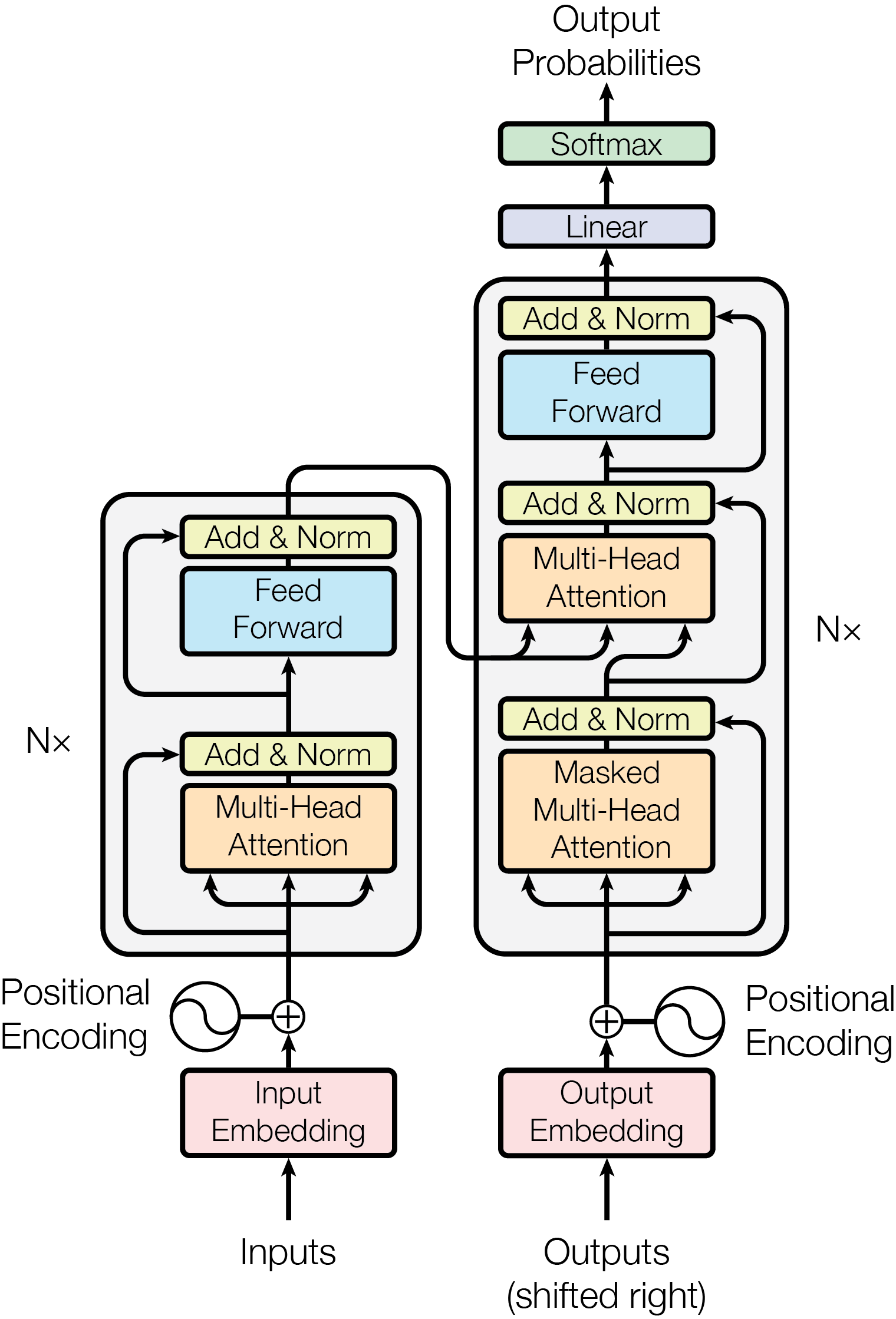
Source and attribution · click image to enlarge
Left: encoder.
Reads the input sentence.
Right: decoder.
Uses the output so far and the encoder’s information to predict the next token.
Embeddings, feed-forward layers and softmax are familiar. We’ll unpack attention first.
Our lesson uses a causal next-token example, not this whole translation model.
What could come next? Use all the words before the blank.
The last three words are the same in both contexts.
all tokens so far ↓
↓ next-token probabilities
$E_{\text{tok}}$ is the learned vocabulary lookup table: one stored row per token.
$t_i$ is the token ID at position $i$. Writing $E_{\text{tok}}[t_i]$ means “read that token’s row from the table.”
The word bank gets the same lookup row wherever it appears.
In a trained model, learning adjusts the table. Here we use hand-chosen rows so we can follow the arithmetic.
One coordinate is one number in the row. $d_{\text{model}}=4$ means four features per token.
Water: water scenes. Finance: money scenes.
Person: people. Glue: function words such as “the” and “and”.
We chose these feature scores and names for teaching. They are not probabilities. Real learned embeddings usually mix features across coordinates without such tidy labels.
| Position 1 | Position 2 | Position 3 |
|---|---|---|
| Maya | helps | Ravi |
| Ravi | helps | Maya |
Maya gets the same lookup vector in both sentences. That vector alone does not tell us whether Maya came first or last.
In Part I, concatenation kept the positions in separate input slots. Here, we’ll give each token row a position cue before the rows interact.
Same word row. Different position row. Add them coordinate by coordinate.
Still four coordinates. These hand-chosen table entries are used throughout the example.
The row selected by token ID $t_i$.
A vector for position $i$.
Their sum, before any contextual update.
The superscript $(0)$ means “before any contextual update.” The result already combines word and position information. The labels describe our illustrative word features, not a clean separation of meaning and position in the sum.
A learned position table has one row per supported position, much like the vocabulary table has one row per token. Here we set its values by hand. The original Transformer also describes fixed sinusoidal vectors. Both designs add vectors of the same width. Other architectures can supply position information differently.
All following bank calculations use these same four-coordinate sums. The named features and the small position offsets are hand-chosen teaching values. Attention and prediction can use the position information because it shares coordinates with the word features.
$\ve{E}$: the hand-chosen bank example
$T=10$
Tokens in this input.
$d_{\text{model}}=4$
Numbers in each token row.
$\ve{E}$ has shape $\htmlClass{sentence-count}{10}\times\htmlClass{sentence-width}{4}$
token rows × coordinates
$\ve{e_6}$ is row 6: river.
One sentence, ten token rows. The blank has no row yet.
We call the number of input tokens $T$. Here we have ten tokens, even though some words repeat. The symbol $d_{\text{model}}$ counts the numbers used to represent each token. In our bank toy, that count is four. So the sentence matrix $\ve{E}$ has ten rows and four columns.
Lowercase $\ve{e_i}$ means the row for token position $i$. For example, $\ve{e_6}=[3.1,-0.1,0.0,0.1]$ is the row for river after adding position 6. Before any contextual update, $e_i=e_i^{(0)}$. Stacking the rows gives $E=[e_1;\ldots;e_T]$, with shape $T\times d_{\text{model}}$. The table shows the starting values from our hand-chosen bank model.
$E_{\text{tok}}$ is the vocabulary lookup table shared across sentences. $E$ holds the rows for this particular input. Contextual updates change the rows of $E$ during the forward pass. Training can change the stored lookup table.
The model works with a row of numbers per token. We judge its prediction by the probability it assigns to the correct next word, so those rows need to carry the relevant context.
What can we predict if the output head receives only the last token?
Baseline: only the last token
Baselines for using context
We have a row of numbers for each token.
How much of the prefix should the predictor read?
We have one starting row per token. These rows have not yet exchanged information.
The fisherman sat beside the river bank and watched the ___
Plausible next word: water
She deposited the cheque at the bank and watched the ___
Plausible next word: teller
How can the earlier clues change the next-word probabilities, even when the ending stays the same?
Start with a model that sends only the last token to the output head. Its entire input is one row of $d_{\text{model}}$ numbers. Switch the context and the bars stay put. The table below explains why: both sentences end with the at position 10, so they supply exactly the same starting row. The same row gives the same probabilities. In this toy, eight candidates also happen to tie. A last-token-only model need not produce a uniform distribution; it must produce the same distribution whenever it receives the same row.
A deliberately limited test: of the ten rows, the output head reads only the starting row for “the”, at position 10.
Only the highlighted position is used.
→
The earlier rows do not reach this prediction. Can it tell the two contexts apart?
Both contexts give the head the same input: “the” at position 10.
We need earlier clues to influence the prediction.
All eight displayed candidates tie at about 0.094 each in this hand-chosen toy. “Other ×12” adds the probabilities of the remaining twelve vocabulary tokens. Full bar = probability 1. The important comparison is between the river and cheque sentences: every individual token keeps the same probability.
Like Part I: input → hidden layer with ReLU → vocabulary scores.
- $\htmlClass{head-input}{e_{10}^{(0)}}$: $1\times4$ input row
- “the” at 10, before context updates.
- $\htmlClass{head-hidden}{h_{10}}$: $1\times8$ hidden row
- ReLU: $\max(0,x)$ for each entry.
- $\htmlClass{head-param}{W_1}$: $4\times8$ · $\htmlClass{head-param}{b_1}$: $1\times8$
- Input → hidden, then ReLU.
- $\htmlClass{head-param}{W_2}$: $8\times20$ · $\htmlClass{head-param}{b_2}$: $1\times20$
- Hidden → scores. One bias per output.
- $\htmlClass{head-score}{\ell}$: $1\times20$ logits
- Called $z$ in Part I; not probabilities.
Each score reads all eight hidden units. Dots omit 16 outputs.
Superscript $(0)$: before context updates. The four inputs are coordinates of one token, not four tokens.
The diagram’s input circles are coordinates of one row, not different tokens. Each hidden unit receives all four coordinates; each score receives all eight hidden activations. A connection can have weight zero. The leading 1 in each shape means one prediction row. There are two learned affine layers, with ReLU between them; the final softmax comes next. Our parameters are hand-chosen illustrations, not trained measurements. In the source code, $W_1,b_1$ are W_hidden,b_hidden and $W_2,b_2$ are W_vocab,b_vocab. For the baseline, all eight hidden activations happen to be zero:
More generally, $t$ is the last input position ($t=10$ here), and $\htmlClass{head-input}{e_t^{(0)}}$ is its starting row. We sometimes write the current row simply as $\htmlClass{head-input}{e_t}$; later it will include information from other tokens. The output-head operation stays the same.
- $\htmlClass{head-score}{\ell}$: all 20 scores
- One for every possible next word. A score may be negative, zero, or positive.
- $\htmlClass{head-prob}{p}$: all 20 probabilities
- For each score $s$, $\exp(s)=e^s$. Divide by the total; probabilities sum to 1.
For our input “the” at position 10, the score for water is :
$p_{\text{water}}$ means “probability that the next word is water.” Both rows $\htmlClass{head-score}{\ell}$ and $\htmlClass{head-prob}{p}$ have shape $1\times20$.
Same input row → same scores → same probabilities. Softmax cannot supply the missing context.
In general, $\htmlClass{head-prob}{p_j}=\exp(\htmlClass{head-score}{\ell_j})/\sum_{r=1}^{20}\exp(\htmlClass{head-score}{\ell_r})$. The indices $j$ and $r$ select vocabulary words, not positions in the sentence. The sum includes every word, including the ones omitted from the network drawing.
In next-token notation, $\htmlClass{head-prob}{p_j}=p(x_{t+1}=v_j\mid x_{\le t})$: $x_{\le t}$ means all tokens supplied so far, $x_{t+1}$ is the next token, and $v_j$ is vocabulary word $j$. Here $t=10$, so we predict position 11. This restricted baseline ignores the earlier tokens despite writing the full prefix after the conditioning bar. It is the model’s prediction, not the true distribution of language.
This baseline reads only the final “the” at position 10 in each sentence.
The four numbers the head receives for “the”
Next: let several recent token rows reach the model.
The output head can only use the row it receives. Earlier words must contribute to that row before the head can use them.
A wider window includes more words, but it still leaves a boundary.
Baseline: a fixed window of w tokens
Give the model more context by concatenating the last $w$ representations into one long row. Both network views use the MLP layout from Part I. Here we choose eight hidden units and twenty vocabulary scores. First identify the available inputs, then join their coordinates, then examine the network's equations and parameters. At $w=3$, river is outside. At $w=10$, every token fits because this sentence is short. Changing the window changes the required parameter shapes. These are architecture sketches, not trained predictions for every window size. The article also derives the optional simpler linear head separately.
Concatenate the previous $w$ token representations into one long vector and predict from that. $w$ denotes the window width; we reserve $K$ for the matrix of attention keys later.
The MLP can use only the words inside its window
Architecture sketch: resizing the window requires a matching weight matrix, not an update to the same trained network.
Behind the boundary means unavailable: no input node, no connection.
c: the concatenated context row.
10: the last input position.
It stays 10 when the window changes.
Scroll horizontally to follow the joined row.
Same numbers, in token order. No summing.
What the dimensions mean
- w
- Token slots in the input window.
- d
- Numbers in each token row. Here, d = 4.
- H
- Hidden neurons. We choose H = 8.
- V
- Words in the vocabulary. Here, V = 20.
W₁ and W₂ hold the learned connection weights between the columns.
The same forward pass as Part I
h = hidden activations. ReLU replaces negative inputs by 0.
ℓ = vocabulary scores. p = their probabilities.
b₁ and b₂ are learned biases added to the weighted sums: one per hidden neuron and per output word.
One weight per connection
| Parameters | Count rule | Here |
|---|
N counts these two layers only. Embedding and position tables are additional.
The input row has shape $1\times wd$. $W_1$ has shape $wd\times H$, $b_1$ and $h$ have shape $1\times H$, $W_2$ has shape $H\times V$, and $b_2$, $\ell$ and $p$ have shape $1\times V$. Training learns the weights and biases. The layer parameter count is $N=wdH+H+HV+V$. Doubling w doubles only the first term, not the entire model. Each additional token slot adds dH weights. This architecture sketch uses the same hidden-layer convention as Part I and does not run a trained MLP for each slider setting.
A simpler linear head
This alternative connects the concatenated input directly to the vocabulary scores. It removes the MLP's hidden layer, so its single matrix W has a different shape from either W₁ or W₂ above.
Linear head · 4 numbers/token · 20 vocabulary words
W = connection weights; b = one bias per word.
ℓ = logits (scores): multiply → sum → add bias.
All 20 scores → 20 probabilities; they sum to 1.
In this direct linear head, each extra token adds 4 inputs and 4 × 20 = 80 weights. The 20 outputs stay fixed.
Click an output circle or focus it and press Enter/Space. Four of the twenty output nodes are shown, in vocabulary order; dots stand for the other sixteen. For windows wider than three tokens, the diagram shows the first two and final token groups and counts the omitted coordinates. Every retained coordinate connects to every output, including nodes hidden by dots. These are architecture sketches: changing w requires a differently shaped weight matrix. No numerical weights or probabilities are invented.
In general, $c_t$ is the concatenated context ending at input position $t$. Here $t=10$, so $p$ predicts the word at position 11. With $d_{\text{model}}=4$ coordinates per token and vocabulary size $|\mathcal V|=20$, $c_t$ has shape $1\times(wd_{\text{model}})$, $W$ has shape $(wd_{\text{model}})\times|\mathcal V|$, and $b$, $\ell$ and $p$ each have shape $1\times|\mathcal V|$. The weight matrix contains $wd_{\text{model}}|\mathcal V|$ parameters, plus $|\mathcal V|$ bias parameters. Each column of W holds the weights for one vocabulary word. Softmax uses all twenty scores, not just the four drawn here.
A window keeps the most recent w tokens. Our original prefix had 10 tokens. These have 20.
River scene: “water” is a plausible next word
Bank scene: “teller” is a plausible next word
Blue = available input. Grey = outside the window. Underlined orange = earlier clue.
Sentences illustrate visibility only, not measured predictions.
We count whitespace-separated words for these illustrative prefixes and leave punctuation out of the token count. Both contain twenty input tokens. At w=10 the input consists of positions 11 through 20: “after a long quiet afternoon turned around and watched the”. The blank is position 21, the token to predict. The first ten words still exist in the text, but this baseline never supplies their rows to the prediction head. With the same visible words in the same positions and the same fixed parameters, the head returns the same probability distribution. Drawing a random next word can differ without making that distribution depend on the unseen clue.
The complete river scene makes “water” a plausible continuation, while the bank scene suggests “teller”. These are examples, not forced answers or measured probabilities. The word river is at position 6 and first enters at w=15. Cheque is at position 5 and enters at w=16. At w=20 both entire prefixes fit. For a 35-token prefix, a window of 20 would keep positions 16–35 and could again miss an important clue at position 6. The window slides with the prediction position rather than cutting every sentence at a fixed absolute position.
Keeping 20 tokens makes river and cheque available in those examples.
| Window | Joined input row | W₁ to 8 hidden neurons |
|---|---|---|
| 10 tokens | 1 × 40 | 40 × 8 |
| 20 tokens | 1 × 80 | 80 × 8 |
Each token still has 4 numbers. The joined row and W₁ grow; W₂ stays the same.
Can we collect useful information from a longer prefix into one fixed-width summary?
The input slots stay fixed
The network can respond to words inside those slots. The limit is which input rows reach it, not an inability to use the content they contain.
Counting the direct linear head
This count belongs to the single-matrix alternative above. It differs from the two-layer MLP's count $wdH+H+HV+V$.
w = token slots, d = numbers per token. V = vocabulary size. Below: d = 4, V = 20. Counts cover the linear head only.
A slot holds one token row, so w slots of d numbers supply wd input numbers. Each input connects to all V outputs, giving wdV weights in W. Each output also has one learned bias, giving V biases. Nhead counts all those learned numbers together.
Read the first row: 10 token slots × 4 numbers = 40 inputs. Each connects to 20 output words, giving 40 × 20 = 800 weights. Add 20 biases to get 820 head parameters. The other rows change only the number of slots.
For a larger illustrative design, d = 128 and V = 10,000:
w = 10: 12.8 million weights. w = 100: 128 million.
More slots cost more parameters. A still longer prefix can put the clue outside again.
For fixed embedding width and vocabulary, doubling w doubles the number of weights in W. The V bias parameters stay fixed, so the head total is not exactly doubled. A trainable token lookup adds Vd parameters independently of the window width. A learned absolute-position table, if used, adds its own parameters based on the supported positions. Neither is included in this head-only table.
For the MLP sketch earlier in this section, the first layer has wdH weights and H biases, where H is the hidden width. Its output layer has HV weights and V biases. Increasing w enlarges the first matrix while the hidden and output widths can stay fixed. The direct linear-head formula above should not be mistaken for the parameter count of an entire transformer.
Next we calculate a mean, inspect what it gives equal importance to, and then try unequal contributions.
Combine all available token rows into one summary whose width stays fixed.
Summarizing the prefix
Summarizing the prefix
The prefix is all tokens up to and including the current input position.
How can they contribute to one fixed-width context summary?
- Averaging. Every available row gets an equal share.
- Hand-chosen weights. We choose each row's share.
- Attention. The model computes shares from the inputs.
We now build context for a token already in the input. Begin at position 7, bank, using the seven known token rows. A pooled summary $m_i$ combines their corresponding coordinates, while the earlier $c_t$ concatenated rows. Try averaging first, then choose unequal contributions yourself. The summary stays four numbers wide. Later, we will build a summary at every input position before prediction. These arithmetic operations do not update the stored vocabulary table.
Before prediction, let input tokens collect context.
Start with bank at position 7: it is already in the input, not a word to guess.
Concatenate
Pool into a summary
Combine matching coordinates. The result stays 1 × 4.
First rule to try: average each coordinate across the available rows.
The seven blocks above are the representations of the seven words, each with four coordinates. Concatenation keeps all 28 entries separately. A pooled summary compresses the available rows into four entries, so more tokens do not increase its width. Combining more rows still takes computation, and compression can lose information. We will call this new summary m, keeping c for concatenation. After learning how to build a summary at one position, we can apply the same idea at each input position before making next-token predictions.
$i$ is the position of the input token whose context summary we are building.
Blue = contributes. Outline = current token. Grey = excluded.
Fixed window, w = 3
Full prefix: all tokens so far
The previous section called window size w. A “last k tokens” rule is the same idea with k in place of w. Both w and k count how many recent input rows we keep. In contrast, i identifies the current input position. At that position a window includes max(1, i − w + 1) through i, while this full-prefix average includes 1 through i. Neither uses positions after i. At i=7, averaging the last three rows would be mathematically valid, but it would discard rows 1–4. Here we deliberately try a summary that lets all seven available rows contribute. Later we will choose their contributions unequally.
For each coordinate, add the numbers from the available rows and divide by the number of rows.
$m_i$ = pooled summary. $i$ = current position. $e_j$ = input row at source position $j$, from 1 through $i$.
Does bank mean a riverside or a financial institution here?
The fisherman sat beside the river bank
Fisherman and river suggest the riverside meaning.
But averaging gives river and “the” equal shares. Should they contribute equally to bank's context?
Let's try unequal shares, giving these useful clues more influence. First, we will choose the shares ourselves.
The highlights express our interpretation of this sentence, not measured attention weights. Words such as “the” can matter for other questions. No exact shares have been assigned yet. Bank is already an input word at position 7, and the task is to gather context for it from the available prefix.
We are still building bank's context at $i=7$. Now give river a larger share.
If we choose a weight of 0.5, multiply every coordinate of river's row by 0.5.
This is river's contribution only. The other six weights must add up to 0.5.
The example chooses 0.5 by hand. It is a single scalar shared by all four coordinates. These weights mix input rows, whereas the output-head probabilities describe possible next tokens. We have not yet introduced a method for computing the weights from the inputs.
For bank, keep $i=7$ fixed. Take a weighted share of each source row $j=1,\ldots,7$.
The sum sign $\sum$ means “add these weighted rows”:
$$\htmlClass{pool-summary}{m_i}=\sum_{j=1}^{i}\va{\alpha_{ij}}\,\ve{e_j}$$$m_i$: the resulting summary.
One row of 4 numbers.
$\alpha_{ij}$: share from source $j$.
One number, for receiver $i$.
$e_j$: the input at source $j$.
One row of 4 numbers.
For this receiver: $\va{\alpha_{ij}\geq0}$ and $\sum_{j=1}^{i}\va{\alpha_{ij}}=1$.
Only sources 1 through $i$ contribute, including $i$ itself. Equal weights $\va{1/i}$ give the mean again.
The raw weights are normalized to sum to 1.
Same output head, then softmax
Predicting position 8, after bank. This untrained head is illustrative. The original sentence continues with and.
Normalized shares sum to 1. Values shown rounded. Calculations use full precision.
Input: The fisherman sat beside the river bank ___ (position 8)
Four context numbers → 8 ReLU units → 20 scores. $\htmlClass{pool-prob}{p}=\operatorname{softmax}(\htmlClass{pool-score}{\ell})$.
A different summary can change the probabilities without changing the top word.
Each row is a separate prediction. This untrained head does not recover the original next word, and.
Probabilities use unrounded summaries and the existing saved vocabulary weights and biases. The rows compare the four saved presets, independent of custom slider values. The live readout on the weight-selection slide also supports custom weights and reports ties. The summary feeds the head directly in this diagnostic baseline. Later attention examples use a contextual update and residual addition, a different input to the same head.
So far, you chose the weights by hand. We need a rule that computes the shares from the input rows.
Which sources are useful for this receiving token?
Receiver: bank at $i=7$. One source: river at $j=6$.
How can the model calculate their weights $\alpha_{ij}$ from the inputs?
The weighted sum is already defined. The next step is a mechanism that computes its weights from the receiving token and the available sources.
Attention computes the shares from the inputs. Search will help us understand how to match sources and retrieve information.
Attention and the search analogy
3. Attention
How does a token gather useful information from its context?
We will compute the weights from the inputs.
For bank at position 7, attention computes how much each available source contributes to its context.
- Compare the receiver with each source.For example, compare bank with river to get a matching score.
- Convert the scores into weights.Higher scores get larger shares. All the shares add up to 1.
- Mix source information using those weights.The result is one fixed-width context summary.
A trained model learns how to compute these weights. A new input can produce different weights.
Attention weights describe contributions to a context summary, not next-word probabilities. During generation, the learned parameters stay fixed while the weights depend on the current inputs. This deck's demonstration parameters were chosen by hand. The distinction between matching a source and returning its information motivates the search example next.
A short detour · three roles we need for attention
Information retrieval
Finding useful information in a collection. Our example: searching for a video.
- Query
- What am I looking for?
- Key
- A description of each source, used for matching.
- Value
- The information that source returns.
Query–key matches will determine the weights $\va{\alpha_{ij}}$.
Then return to bank and river: use those weights to mix values.
We will first express several questions as query vectors. Each coordinate has a named topic in this example, and a larger number represents a stronger request for that topic. After comparing the questions, we will describe videos on the same axes, then calculate which descriptions best match the request. These numerical examples are chosen by hand to make the roles visible. Learned representations do not generally have one human-readable topic per coordinate.
A user asks a video site a question. That request is the query.
What are we looking for?
Represent the request with four numbers in a fixed order.
- 1. Gradient flow
- How derivatives travel backwards through layers.
- 2. Optimisation
- How we use gradients to update weights.
- 3. Architecture
- How a network's layers are structured.
- 4. Generalisation
- How a model avoids overfitting to training data.
A larger number means a stronger request for that topic. These are not probabilities.
We choose the axes and numbers by hand. Learned coordinates need not have these names.
$\vq{q}$ is one row of four numbers: $1\times4$. Underlined numbers mark the strongest topic.
Every request uses the same axes in the same order.
The question changes the row. Its width stays four, even when the question has more words.
Video 1: Backpropagation
The chain rule applied layer by layer, from the loss back to every weight.
Which topic does this video cover most strongly?
Its key describes the source: gradient flow is the main topic.
Query: what the learner wants. Key: what the video covers.
Video 1: Backpropagation. One description, four topic strengths.
2.2 under gradient flow is strongest. Optimisation 0.6 and architecture 0.2 are smaller. Generalisation is 0.0.
$\vk{k_1}$ means the key of video 1. It has the same $1\times4$ shape and axis order as $\vq{q}$.
Only the request row changes. Every video key keeps its four numbers.
Multiply matching coordinates, then add: $s_j=\vq{q}\cdot\vk{k_j}$.
For this matching step, the site uses only the dot product between the query and each key.
$$s_j = \vq{q}\cdot \vk{k_j}$$$\vq{q}$ = query representation, $\vk{k_j}$ = key of item $j$, $\vv{v_j}$ = value of item $j$.
Values: what a source sends
Query–key scores tell us which sources match.
What information should we get back from a matching source?
Query:
Key: why this video matches
Its topic description signals .
Compare this description with the query. It helps select the video; it does not yet explain the topic.
Value: information from this video
Illustrative transcript · written for this example
The key helps find the source. The value represents what we take from it. Next, we will express that information as numbers.
Query: “How can I contact or visit the library?”
| Key: contact to match | Value: four fields returned together | |||
|---|---|---|---|---|
| Extension | Floor | Opens | Closes | |
| Library | 204 | 2 | 09:00 | 20:00 |
| Admissions | 118 | 1 | 10:00 | 17:00 |
The key finds Library. Its value lets us dial 204 or visit floor 2 between 09:00 and 20:00.
A changed opening time updates one value field. The key can still be “Library”.
Fictional exact lookup. Attention combines numerical feature vectors, not literal contact fields.
Maya cycled home in the rain. Cold and tired, Maya reached for a hooded red wool coat. She …
Query from “she”: “Which earlier person could I refer to?”
| Source | Key: matching clues | Value: details it can send |
|---|---|---|
| Maya | Person, singular |
|
| coat | Object, singular |
|
Knowing Maya is cold and tired can help continue the story: “She went inside to rest.”
Illustrative later-layer vectors. Earlier layers have gathered these facts. The real vectors contain numbers.
Maya cycled home in the rain. Cold and tired, Maya reached for a hooded red wool coat. It …
Query from “it”: “Which earlier object could I refer to?”
| Source | Key: matching clues | Value: details it can send |
|---|---|---|
| Maya | Person, singular |
|
| coat | Object, singular |
|
Same keys and values, a different query. Now the colour and material can help continue: “It was made of red wool.”
A possible continuation, not a measured prediction. Attention mixes numerical features from the sources.
Query and key each have four matching coordinates for their dot product. The value has eight content coordinates; we do not dot it with the query.
Hand-chosen strengths: 0 = no signal, 1 = strong signal. They need not sum to 1. Learned coordinates need not have these names.
The same eight content features for every video
$\vv{v_j}$: one $1\times8$ row per video, reused throughout retrieval. Values can share width and information with keys. Their use differs; eight is our choice here.
Question:
Same eight hand-chosen strengths. Bold entries link to the teal ideas in the explanation.
The text spells out the source's content for the reader. In the numerical retrieval calculation, the result is the entire value row. The row is an illustrative representation of that content, not a way to reconstruct the English explanation. Later, soft retrieval will combine value rows rather than combine sentences.
What am I looking for?
When should you retrieve me?
What information do I send?
The query comes from the learner's question. Each stored video has a key for matching and a value for returning information. These are the same hand-chosen example vectors used in the preceding tables. The coordinate lists above represent rows, not new column-vector conventions. Matching bars run from 0 to 2.5, while content bars run from 0 to 1.
Only the query and key determine the match score. Once we choose an item, we retrieve its value.
Return one best match, or mix information from several? Use the same gradient question (query 1), keys and values to compare.
Hard retrieval → soft retrieval
Hard retrieval returns the value of the highest-scoring item. Attention blends values according to how well their keys match the query. Follow that calculation in the tables: softmax converts the previous section's scores into the $\va{\alpha_j}$ weights, each weight scales its value row, and the bottom row adds the results. Start in hard mode, where one item gets all the weight. Switch to soft mode and lower the temperature to see it approach hard retrieval. The returned row is a mixture of values.
Soft retrieval
Hard retrieval returns one source’s value.
How can several sources contribute to one answer?
Compare the query $\vq{q}$ with each video's key $\vk{k_j}$. Return the winner's value $\vv{v_{j^*}}$.
$$j^* = \arg\max_j\, \underbrace{\vq{q}\cdot \vk{k_j}}_{\text{match score}}, \qquad \text{return } \vv{v_{j^*}}$$Here $j$ is a video index. $\arg\max_j$ picks the winning index $j^*$.
In plain words: choose the video that best matches the question, then take information from that video only.
For our gradient question, Backpropagation wins. Return its entire eight-number value row. The other five videos contribute nothing.
Same gradient-information query $\vq{q}$, same six video keys $\vk{k_j}$.
Each score is $\va{s_j}=\vq{q}\cdot\vk{k_j}$, with $j$ identifying the video.
Backpropagation ($j=1$):
$\va{s_1}=\vq{2.0}\times\vk{2.2}$ ${}+\vq{0.6}\times\vk{0.6}$ ${}+\vq{0.2}\times\vk{0.2}$ ${}+\vq{0.0}\times\vk{0.0}=\va{4.8}$.
First exponentiate each score: $s_j\mapsto e^{s_j}$.
Then divide each result by the same total:
Same eight value coordinates. Displayed numbers are rounded. The sum uses unrounded weights.
One $1\times8$ row, on the same eight content axes.
In soft mode the weights are $\va{\alpha_j} = \operatorname{softmax}_j(s_j/\tau)$. A small $\tau$ makes the mixture sharper. As $\tau \to 0$, soft retrieval becomes hard retrieval when one score is strictly the largest; tied top scores keep sharing the weight. $\tau = 1$ is the formula above.
The query describes what the searcher needs. Keys help score the matches; values carry the information to return. Softmax gives us the weights for mixing that information. We can use the same roles for tokens in a sentence.
The scores determine the weights, which determine the mixture.
Each token supplies a key for matching and a value to send, just as the search results did.
Every token becomes a searchable record
The video example keeps eight content coordinates throughout retrieval. For the sentence arithmetic, we return to our original smaller model: three query/key coordinates and two value coordinates. The matching and mixing rules stay the same.
First take the numerical queries, keys and values as supplied examples. Read their named axes and use them to collect context. After we have followed the message through the residual addition and into prediction, Section 11 explains how these exact same rows are produced from the token representations.
These are hand-designed teaching coordinates, not measured human concepts or axes that real models must learn. The same numerical model supplies every table; nothing is re-sampled between slides.
Back to next-word prediction
The fisherman sat beside the river bank and watched the ___
She deposited the cheque at the bank and watched the ___
Same ending, different clues. How should the next-word probabilities change?
Use attention to collect context from tokens, not videos.
Earlier: the last token alone missed clues. Concatenation grew with the window. Pooling kept a fixed width, but we chose the shares by hand.
Now build context for bank, position 7, using input tokens 1–7.
- 1. Match
- Compare bank's query $\vq{q_7}$ with every available key $\vk{k_j}$, including river's.
- 2. Weight
- Softmax turns those scores into shares $\va{\alpha_{7j}}$. We compute them from the inputs.
- 3. Mix
- Multiply each value $\vv{v_j}$ by its share, then add:
$\vm{m_7}=\sum_{j\le7}\va{\alpha_{7j}}\,\vv{v_j}$, the context collected for bank.
Bank is already an input word. Later, repeat this at the final the (position 10), update its row, and predict word 11.
Bank could mean a river bank or a financial bank. What kind of setting am I in?
A supplied query: what bank is looking for
Take these illustrative numbers as given for now. First use them; later we will explain how the model produces them.
Supplied keys: what each source offers for matching
River offers water-setting evidence. Bank asks for setting evidence. Their matching coordinates can be compared.
Supplied values: the information each source sends
River sends mainly water-scene information. Each value has two coordinates; the matching query and keys have three.
Bank remains the receiver. Inspect one source:
Key: compare with bank's query
Value: send this information
Bank has one query and seven available sources. First choose the weights, then collect the information.
Two jobs: choose weights, then mix values
We will work through attention in two phases. Phase A uses queries and keys to score the available tokens, then turns those scores into weights that sum to one. Phase B multiplies each source's value by its weight and adds the results. The keys help choose where to read; the values carry the information.
Run phase A and click a key in the diagram to inspect its dot product, coordinate by coordinate. Then run phase B and follow each coordinate into the sum. Switch between the original value rows and the $\va{\alpha}\vv{v}$ products to see what the weights changed.
Take “bank” (token 7) as the query in The fisherman sat beside the river bank. First choose where to read. Then mix what those sources send.
Phase A: compare $\vq{q_7}$ with every $\vk{k_j}$ to choose seven weights.
Phase B: use those weights to mix the seven $\vv{v_j}$ rows.
$\vq{q_{7}}$ against every key $\vk{k_j}$: one score per row, then softmax turns the scores into weights $\va{\alpha_{7j}}$
Hold $\vq{q_7}$ fixed; compare it with seven $\vk{k_j}$ rows
The same seven numbers: score → exponential → normalized weight
For each source position $j$:
This produces one scalar score. We repeat it for $j=1,\ldots,7$.
scores = (q_bank @ K.T) / math.sqrt(K.shape[-1])Compare all seven scores:
alpha = scores.softmax(dim=-1)Bank’s query is held fixed; choose a key to inspect its score
Weight shading: absolute 0–1 scale
Scroll sideways to see all seven keys.
One edge from the routing picture, written out
The keys were used to compute the weights; they are not added into this message. All displayed numbers are rounded, while the calculation uses full precision.
m_bank = alpha @ V # [7] @ [7, d_v] → [d_v]Optional: changing values with fixed weights
Keys choose matches; values carry information. Their roles remain distinct even if some numbers happen to be equal.
Set only the values’ “says finance” coordinate to zero. Keep the query and every key fixed. Predict which numbers below will change, then try the switch.
The resulting message
V_alt = V.clone(); V_alt[:, 1] = 0
m_alt = alpha @ V_alt
The query and keys determine the weights. With those held fixed, changing values can change the message without changing the weights.
Queries and keys gave us the weights $\va{\alpha_{7j}}$; the weighted values gave us the message $m_7$. Bank's representation is still unchanged. Next we will turn that message into an update.
How does the retrieved message $m_i$ change the token's representation?
The contextual update Δe
The message $m_7$ is a mixture of values, so it has $d_v$ value coordinates. To add it to bank's representation, we need $d_{\text{model}}$ representation coordinates. $W_O$ performs that mapping and gives us $\vd{\Delta e_7}$. The residual connection adds this update to the original $\ve{e_7}$, combining bank's existing representation with context.
Press Play or advance one step at a time to follow the diagram. The next table shows the numerical result; hover a cell in the final row to inspect the addition. Watch the axis names change at $W_O$: it maps the message's value coordinates into representation coordinates. Attention computes the update, and the residual connection adds it.
Updating the token representation
The weighted values give us a message.
How do we add that message to the token’s existing representation?
The message has 2 numbers. We need a 4-number update to add to bank's embedding.
1. Mix the value rows
$$\underbrace{\vm{m_7}}_{1\times 2}=\sum_{j\le 7}\va{\alpha_{7j}}\,\vv{v_j}$$2. Map into embedding space
$$\underbrace{\vd{\Delta e_7}}_{1\times 4}=\vm{m_7}\,W_O$$3. Add to the original
$$\vp{e_7^{\text{new}}}=\ve{e_7}+\vd{\Delta e_7}$$Here $d_v=2$ and $d_{\text{model}}=4$. Each output coordinate can combine both message coordinates. This diagram uses the same hand-chosen projection as our numerical example.
The attention branch computes an update; the residual branch preserves $\ve{e_7}$
Inside bank's attention update
Follow token 7, bank, through one attention update
The numerical result of the eight-step path
Message → representation-space update → residual addition
In a trained model, $W_O$ learns how to map the message $\vm{m_7}$ into an update $\vd{\Delta e_7}$ with the embedding's required dimensions.
Each update coordinate can combine both message coordinates. The update now matches the shape of the embedding $\ve{e_7}$, so we can add them.
Optional: the fixed matrix used in this worked example
Our illustrative $W_O$ is hand-chosen, with simple entries so the arithmetic is easy to check. Every column mixes both message coordinates. The four columns use different coefficients, including negative ones.
Here “projection” means a linear map into embedding space. It need not be an orthogonal projection. An affine version would add a bias, $\vd{\Delta e_7}=\vm{m_7}W_O+b_O$; this toy uses no output bias.
The example's $d_v\times d_{\text{model}}$ output projection
PyTorch · $m_i$ is $1 \times d_v$; $\Delta e_i$ and $e_i$ are $1 \times d_{\text{model}}$.
delta_e_i = m_i @ W_O
e_new_i = e_i + delta_e_i
The final the (10) now reads tokens 1–10 with its own query. Its context gives a new row:
Same prediction head, different context. These probabilities come from the updated final row, not directly from bank's message.
This small model uses our 4 → 8 → 20 MLP predictor. This prediction head is distinct from the feed-forward sublayers inside a full Transformer.
In $\vp{e_7'} = \ve{e_7} + \vd{\Delta e_7}$, the right branch computed the update and the left branch carried $\ve{e_7}$ unchanged. They meet at the addition: the residual connection.
Bank starts with the same vector in both sentences. Its context gives it different updates.
“bank”: same start, different context
Run the same calculation for the river sentence and the cheque sentence, following bank in both. Its starting row is identical because its token and position are the same. Compare the $\va{\alpha_{7j}}$ columns: river gets most of the weight in sentence A, while cheque and deposited get most in sentence B. Follow those contributions into the message at the bottom and the $\vd{\Delta e}$ row. The update adds water information in A and finance information in B. Drag the slider to add it gradually. The same starting representation becomes context-dependent because it receives different information.
Both sentences put bank at position 7. Its starting representation $\ve{e_{\text{bank}}^{(0)}}$ is the same row in both: same token embedding, same position. Attention is causal, so bank reads itself and the tokens to its left (tokens 1 to 7). The words after it play no part.
Sentence A and sentence B, side by side
Compare the weight columns, then the incoming messages in the footers.
Same initial row + different incoming update
Same initial row + the cheque-context update
Look at the two arrows: they leave the same blue dot and end far apart. The slider adds the update gradually; the comparison tables follow it.
Bank reads only itself and earlier tokens. Words after it contributed to neither update. The two $\vp{e_{\text{bank}}'}$ rows differ because the values and weights across those seven source positions differ.
We have used the rows to gather context and predict. Now explain how the model produces those rows.
Where do queries, keys and values come from?
Queries, keys and values come from projecting the current representation. They are not separate learned lookup tables. Pick a token and compare the four rows: three fixed matrices turn the top $\ve{e}$ row into the query, key and value below it, without changing that input row. Their axis names describe different roles: what the token asks for, when it is a useful match, and what it sends. The matrices below are shared by every token. Step through the lifetime diagram to see when the rows are computed and used. These working vectors help produce $\vd{\Delta e}$; the row passed to the next sublayer is $\ve{e} + \vd{\Delta e}$.
Learning queries, keys and values
We have used supplied vectors to gather context and make a prediction.
How can the model produce those vectors from each token’s current row?
Recover the supplied rows from the current token representation. Every token uses the same three projection matrices:
$$\ve{e_i} \;\rightarrow\; \begin{cases} \vq{q_i} = \ve{e_i}\,W_Q \\[2pt] \vk{k_i} = \ve{e_i}\,W_K \\[2pt] \vv{v_i} = \ve{e_i}\,W_V \end{cases}$$The matrices are learned parameters, fixed during a forward pass. The rows are recomputed from the input; none replaces $\ve{e_i}$. Our example uses hand-set parameters.
Maya cycled home in the rain. Cold and tired, Maya reached for a hooded red wool coat. She …
| Mapping | Input token row | Output, explained in words |
|---|---|---|
| $W_Q$: query | “she” | Which earlier person could I refer to? |
| $W_K$: key | Second “Maya” | Person, singular. A candidate for “she”. |
| $W_V$: value | Same Maya row | Maya cycled home in rain. She is cold and tired. |
Asking for a person and being a person candidate are different signals. Separate query and key mappings can learn each signal. The value mapping chooses which details to send.
Q and K have equal width for the dot product. Their matrices can still learn different weights.
Illustrative later-layer vectors, described in words. Every token uses the same three matrices.
The same source row can serve different purposes. From Maya's current row, $\vk{k_{\text{Maya}}}=\ve{e_{\text{Maya}}}W_K$ extracts matching features and $\vv{v_{\text{Maya}}}=\ve{e_{\text{Maya}}}W_V$ extracts content to contribute. Returning only “person, singular” would leave out the cold and tired state that could help with a continuation such as “She went inside to rest.” That continuation is not an input to this attention calculation.
In the earlier coat example, “it” can produce an object query. The coat's key can match that request, while its value carries red, wool and hood information. The model reuses the same $W_Q$, $W_K$ and $W_V$ matrices for both examples. Each token has all three working vectors, even though the table shows only those involved in one retrieval.
Equal dimensions allow comparison. $W_Q$ and $W_K$ both have shape $d_{\text{model}}\times d_k$, so their output rows align for a dot product. They can still learn different entries. We could tie their weights, but that would restrict the matching function. A value may share information with a key or query. Separate roles do not require completely separate content.
Why a separate value mapping? $\vv{v_j}=\ve{e_j}W_V$ chooses what information to send, rather than what helps match. $W_V$ has shape $d_{\text{model}}\times d_v$. The scalar $\va{\alpha_{ij}}$ multiplies every coordinate of $\vv{v_j}$, so $d_v$ need not equal $d_k$. Within a head all source values must have the same width so we can add them. A value may share information with a key; the roles do not require disjoint features, different numerical values, or different widths.
Holding Q and K fixed while changing V leaves this attention operation's match scores unchanged, but changes the retrieved message. During training, all three mappings learn together from the downstream loss. These are learned feature combinations, not manually assigned labels.
Pick a token. The top row is the only input. Each lower row is that row times its shared projection: $W_Q,W_K$ produce $d_k$ matching coordinates; $W_V$ produces $d_v$ value coordinates. Read the axis names above the cells.
q and k share the same three columns because the dot product compares them column by column. v has its own two columns, and its own width, because it is only mixed and sent.
The three matrices, shared by every token
Four input coordinates, before attention.
The shared query matrix $\vq{W_Q}$
Four rows match the input axes.
Three columns form the query axes.
Input row on the left, matrix on the right. Each matrix column gives one query coordinate.
The receiver's row becomes its query: what information to look for.
The source's row becomes its key: when this source could help.
Same source row, different weights: the value is what this source sends.
Lifetime inside one attention layer
Step through the layer and watch which rows exist at each moment: $\ve{e_i}$ persists, $\vq{q_i}, \vk{k_i}, \vv{v_i}$ are computed and used, $\vd{\Delta e_i}$ is added to $\ve{e_i}$.
The strip scrolls sideways on narrow screens; the lit column follows the stepper.
From the input row to its contextual update
The three projections sit in the second box; they are inputs to attention, and only $\vd{\Delta e}$ comes out of it.
$\vq{q}$, $\vk{k}$ and $\vv{v}$ are working vectors made from the token representation $\ve{e}$. Attention returns $\vd{\Delta e}$, which the residual connection adds to that representation.
Wider query and key vectors can produce a wider spread of scores. Dividing by $\sqrt{d_k}$ controls that scale.
Why divide by $\sqrt{d_k}$?
We first inspect random query/key entries, then repeat the calculation over many pairs to measure the spread. A two-key example connects that spread to softmax saturation. These demonstrations use separate illustrative numbers. The final table returns to our actual bank query. Extra reading below includes the variance derivation, a fixed-score divisor slider and a standard-normal simulation.
Scaling the attention scores
The query–key dot products determine the softmax weights.
Why do we divide each score by the square root of the query/key width?
Earlier, we divided our three-coordinate scores by $\sqrt{3}$. Here is why, using random vectors.
Each entry is an independent fair choice: −1 or +1. Read the first 2, 4, or all 8 coordinates.
Some terms cancel. One pair cannot establish a trend, so we will repeat this with many random pairs.
Draw fresh $\vq{q}$ and $\vk{k}$ with independent −1 / +1 entries. Multiply matching entries and add.
Bar height = % of draws at that score. Standard deviation (SD) measures the horizontal spread. Both rows use the same axes.
The same experiment, completed for four widths: 3,000 pairs each. Standard deviation (SD) measures the typical distance from the mean.
All coordinates: independent, mean 0, variance 1. Both bar columns use the same 0–17 scale.
Raw spread grows roughly like $\sqrt{d_k}$. Dividing by that factor keeps it near 1 in this experiment.
In our simple ±1 example: $X_l=q_lk_l$ is equally likely to be −1 or +1. Its mean is 0 and its squared distance from 0 is always 1, so its variance is 1.
A whole score: $s=X_1+\cdots+X_{d_k}$. For independent products, the variances add:
$$\operatorname{Var}(s)=\underbrace{1+\cdots+1}_{d_k\text{ terms}}=d_k$$SD is the square root of variance: width 4 gives SD 2. Width 16 gives SD 4.
$$\operatorname{SD}(s)=\sqrt{d_k}\qquad\operatorname{SD}\!\left(\frac{s}{\sqrt{d_k}}\right)=1$$Other distributions work too. Independent query/key coordinates with mean 0 and variance 1 (e.g. standard normal) give the same result. Their squared product averages 1. Learned vectors need not obey these assumptions exactly.
One query, keys A and B, $d_k=64$. First, use the raw scores. Softmax exponentiates each score, then divides by the sum of both exponentials.
Almost all the weight goes to B. A's weight is tiny, but still positive. The two unrounded weights sum to 1.
The scaling factor is $\sqrt{64}=8$: $-8/8=-1$ and $8/8=1$. Now repeat the same softmax calculation.
B still gets more weight. The score gap fell from 16 to 2, so A now contributes meaningfully too.
The two calculations, side by side. Dividing by $\sqrt{64}=8$ changes the score gap and the weights. B remains the winner.
The learning problem: softmax saturation. Near 0 or 1, the weights respond weakly to small score changes. Gradients through attention can become tiny, making queries and keys harder to adjust.
Overflow is separate. Stable softmax subtracts the largest score to keep exponentials safe. That leaves the score gaps unchanged.
The variance argument
Assume all query and key coordinates are mutually independent, mean 0, variance 1. Each product $q_lk_l$ has variance 1. Adding $d_k$ independent products gives
$$\operatorname{Var}(\vq{q}\cdot\vk{k})=d_k,\qquad\operatorname{SD}(\vq{q}\cdot\vk{k})=\sqrt{d_k}.$$Dividing by $\sqrt{d_k}$ makes the variance 1 under those assumptions. Learned coordinates need not obey them exactly. Scaling controls the expected size of the scores, but attention can still be sharp.
Stable softmax uses $\exp(s_j-\max_l s_l)$. Subtracting one constant preserves every score difference and probability. Scaling divides those differences, so it changes the probabilities. These operations solve different problems.
scores = (Q @ K.T) / math.sqrt(Q.shape[-1])
alpha = scores.softmax(dim=-1)
Four fixed raw scores, with and without scaling illustrative numbers
Hold the raw scores $r=[0,0.5,1.5,-0.5]$ fixed. The scaled scores are $s=r/\sqrt{d_k}$. Increasing the divisor flattens softmax(scaled), while softmax(raw) stays fixed.
Gaussian check: score variance across dimensions
Read down the first column: the variance of the raw dot product tracks $d_k$. The second column stays near 1.
In the toy model (dk = ): bank reading the first 7 tokens
Same four columns, real numbers. The note in the following block says how much the factor $\sqrt{d_k}$ changes the top weight.
River still wins. Scaling reduces the score gaps, so softmax is less concentrated.
scores = (q_bank @ K.T) / math.sqrt(K.shape[-1])
alpha = scores.softmax(dim=-1)
Scaling counteracts the expected growth with dimension. Learned vector lengths and alignment still affect score differences, so attention can remain sharp.
A next-token prediction may use the prefix, but it must not read the answer.
Causal masking
During training, the answer for position $i$ is already in the sentence at position $i+1$. We need to stop the model from reading it. Toggle the causal mask and watch row 5. With the mask on, token 5 (the) reads only positions 1 to 5. With it off, much of its weight moves to future tokens: river is the immediate target, and bank provides further future information. Send the values in both states and compare the messages. The mask enforces $j \le i$ by setting forbidden scores to $-\infty$ before softmax.
Causal masking
Each position predicts the next token.
How do we prevent it from reading future tokens during training?
Example: position 5 (“the”) predicts position 6 (“river”)
| Allowed input: positions 1–5 | Target: position 6 | Later |
|---|---|---|
| The fisherman sat beside the | river | bank … |
During training
The full sentence is available. The mask hides river and all later words from position 5. We use “river” to check its prediction.
During generation
We have only the five-word prefix. The model predicts a next word, then we append it. The future words are not available.
When scoring a full test sentence, we keep this same mask.
Every position predicts its next token at the same time
Training does not run one query at a time. One pass through the sentence scores every position at once: each token is a query, reads the tokens up to itself, and is graded on the token that follows it.
Short sequence shown; the ten-token sentence continues the same staircase. Position $i$ may read tokens $1 \ldots i$ and must predict token $i+1$.
Each is a $10\times10$ table. Row $i$ is the receiving token. Column $j$ is the source token.
| $S$: match scores |
$$S_{ij}=\frac{\vq{q_i}\cdot\vk{k_j}}{\sqrt{d_k}}$$
Query $\vq{q_i}$, key $\vk{k_j}$, matching width $d_k=3$. |
|---|---|
| $M$: causal mask |
A fixed position rule: 0 keeps the score. $-\infty$ blocks a future source. |
| $\va{A}$: attention weights |
Softmax each row. $\va{A_{ij}}=\va{\alpha_{ij}}$ weights the source's value $\vv{v_j}$. |
Receiver: position 5, “the”. Its target is position 6, “river”. Columns below are source positions $j$.
Softmax exponentiates, then divides by the row total. Since $e^{-\infty}=0$, river's final weight is zero.
The same rule for four positions
Rows are receiving queries $i$. Columns are source keys and values $j$. A check allows that source, including the diagonal. A cross blocks a future source.
Start with every query-key score:
$$S=QK^\top/\sqrt{d_k}$$Add $M_{ij}=-\infty$ wherever $j>i$.
Then $e^{-\infty}=0$, so those attention weights are exactly zero.
scores = scores.masked_fill(future, float('-inf'))
weights = scores.softmax(dim=-1)
The real attention matrix $\va{A}$ for sentence A (10 tokens), with the mask on or off
Toggle the mask and watch the hatched triangle: with the mask off, weight moves into it, and the outlined cells $(i, i+1)$ are where each token could read its own answer. Click any cell for the score arithmetic behind its weight.
Hover a cell to read one weight.
One leak, up close: token 5 (“the”) whose next token is “river”
Compare the two rows: the mask-off row can read its immediate target, river, and other future tokens such as bank. Press the button to see which tokens send.
The loss asks for $p(x_{i+1}\mid x_{\le i})$.
Without the mask, the representation at $i$ can contain $x_{i+1}$ itself.
That shortcut disappears at generation time, exactly when the model must work.
The rows still sum to 1 with the mask off. To find the leak, check which positions received weight, not just the totals. Causal masking keeps next-token training restricted to information that will also be available during generation.
How does the updated representation change the next-token probabilities?
From Δe to the next-token probabilities
Sections 09 to 13 built an updated vector for bank. Now extend the prefix through “and watched the” and predict the token after that final the. Its query, not bank’s query, determines this attention row. In this single-layer toy, earlier words reach the prediction through the update to that last position. Switch the context between the river and cheque sentences: the attention row, update and probabilities change. Then bypass attention and switch again: the probability row stays fixed, just as in section 02.
The known prefix now has ten tokens. The final the supplies $\vq{q_{10}}$; we predict what follows it. Bank’s earlier query $\vq{q_7}$ is not reused.
Earlier: bank at position 7 received context through $\vq{q_7}$.
Now: the at position 10 receives context through $\vq{q_{10}}$.
The next token is still unknown. It cannot supply the query.
q_last = E[-1] @ W_Q # the current last known positionPredicting the next token
Attention can collect context without looking ahead.
How does the final input token use that context to predict what comes next?
The same starting “the” gives the same query in both contexts
Toy meaning: ask for water or finance clues. The query alone does not know which scene.
$r_j=q_{10}\cdot k_j$
$s_{10,j}=r_j/\sqrt{d_k}$
$\alpha_{10,j}=\operatorname{softmax}(s_{10,:})_j$
scores = (q_last @ K.T) / math.sqrt(K.shape[-1])
alpha = scores.softmax(dim=-1)  # ten source weights; sum = 1
One source's contribution
All ten weighted values together
Sum of all ten contributions.
Project the message, then add it: $\vd{\Delta e_{10}}=\vm{m_{10}}W_O$
$m_{10}=\alpha_{10,:}V$
$1\times d_v$
$\Delta e_{10}=m_{10}W_O$
$1\times d_{\rm model}$
$e'_{10}=e_{10}+\Delta e_{10}$
$1\times d_{\rm model}$
delta_last = (alpha @ V) @ W_O
e_last_new = E[-1] + delta_last
The output head: logits, then probabilities
$h_{10}=\operatorname{ReLU}(\vp{e_{10}'}W_1+b_1)$
$\ell=h_{10}W_2+b_2,\qquad p=\operatorname{softmax}(\ell)$
This softmax is over next-token candidates, not the source positions used by attention.
One weight per known source position.
One probability per possible next token.
h = (e_last_new @ W_hidden + b_hidden).relu()  # W1, b1: 4 → 8
logits = h @ W_vocab + b_vocab  # W2, b2: 8 → 20
p_next = logits.softmax(dim=-1)
The causal chain
Watch the boxes light up in order when you change the context. Earlier tokens reach the head only through the update they send to the last token.
Forward computation changes the token states for this input. It does not change the stored projection matrices or embedding table.
$\ve{e_7}\rightarrow\vv{v_7}$
The final the can read bank’s input-derived value.
$\vp{e_7'}\rightarrow$ new key and value
The updated bank representation becomes a new layer input.
Parallel updates do not read one another’s newly updated rows.
The head reads one row, $\vp{e_t'} = \ve{e_t} + \vd{\Delta e_t}$. In this toy, earlier tokens reach that row through $\vd{\Delta e_t}$; the head does not read them directly.
Follow one complete forward pass, with the numbers visible at every step.
Optional numerical walkthrough
Put the stages together for the ten-token sentence. Each table has one row per token and one column per coordinate, with the result in the last column or bottom row. The numbers come from the same calculation we have worked through by hand. Click a score or press Show the arithmetic to inspect it. At step 3, choose a different query token and advance again. The scores, mask and weights change, while the operations stay the same: score the sources for one query, mix their values, then project and add the update.
Ten tokens, one query, eighteen steps. Press Next step and watch each stage produce its numbers. The pipeline shows where you are in the chain $\ve{e} \to \vq{Q},\vk{K},\vv{V} \to \text{attention} \to \vd{\Delta e} \to \vp{e + \Delta e}$.
Use Next step to inspect the numbers, or presentation Next to continue to the flowchart.
Steps 4 to 17 run for every token at once. We follow one receiver here so that we can inspect each number.
Matrix products run the same calculation for every token at once.
The full attention calculation
The walkthrough followed bank through attention. Every token applies the same operations to its own row, so we can compute them together with matrix products. Here we use the short seven-token prefix: each product carries out the corresponding walkthrough step for all seven tokens.
Follow row 7 as you advance through the operations. It contains bank's numbers at every stage. Each matrix row belongs to a token, and $\vp{E'} = \ve{E} + \vd{\Delta E}$ adds all their updates at once.
The complete attention calculation
We have followed one query from matching to an updated token row.
How do these steps fit together for every token?
Stack the current row representations of the short seven-token prefix as one matrix. Every row of $\ve{E}$ is one $\ve{e_i}$; every operation from section 15 now happens for all $T$ rows in a single product.
$$\ve{E} = \begin{bmatrix} \ve{e_1} \\ \vdots \\ \ve{e_T} \end{bmatrix}, \qquad \vq{Q} = \ve{E}\,W_Q, \quad \vk{K} = \ve{E}\,W_K, \quad \vv{V} = \ve{E}\,W_V$$Dimensions, always in view
Every matrix with $T$ rows has one row per token; row 7 is bank in all of them.
One matrix operation at a time
Row labels are tokens, column labels are the named coordinates. The outlined row is bank, the section 15 computation. Click any score cell for its arithmetic.
Stack one token per row: $\vq{Q}=\ve{E}W_Q,\ \vk{K}=\ve{E}W_K,\ \vv{V}=\ve{E}W_V$.
$M$ blocks future positions. Each row of $\va{A}$ sums to 1; each row of $H$ is that receiver's message. $W_O$ maps it back to model width before addition.
Use the weights, then preserve the input
Each row of $H$ is one receiver’s weighted mixture. $W_O$ returns it to model width before the residual addition.
PyTorch · matrices are row-major; mask contains 0 or −∞.
A = (Q @ K.T / d_k**0.5 + mask).softmax(dim=-1)
E_new = E + (A @ V) @ W_O
The matrix form collects the same calculations into rows. Row $i$ of $\vp{E'}$ is $\ve{e_i} + \vd{\Delta e_i}$. Softmax runs independently on each row, and the mask prevents row $i$ from reading columns $j > i$.
We count the work of concatenation, averaging and attention in optional Part 2B: the cost of a longer context, after studying training and cached generation.
Compare attention with the fixed window (03), mean pooling (04) and fixed positional weights.
Alternatives, position and order
The fixed window and plain mean use fixed inclusion or pooling rules, although their outputs still depend on the words they receive. Compare them with distance-based weights and attention in one table.
Switch between the river and cheque sentences. The first three rows stay fixed because their inclusion or weighting rules do not read the content. The attention row gives more weight to different clues for the blank. Of these four schemes, only attention computes its mixing weights from the words.
All four schemes use $\ve{e_1},\ldots,\ve{e_t}$ to supply information to the last token, $t = 10$. How does each scheme choose what to include or how much weight to give it? Switch the sentence and compare the rows.
Four weighting schemes, one table
Look at the last row: its weights favour different evidence, and only that weight row changes when you switch the sentence.
What each scheme does with the context
| Scheme | Context for the last token | Who sets the weights | What is retrieved |
|---|---|---|---|
| Fixed window | $c_t = [\ve{e_{t-w+1}};\,\ldots;\,\ve{e_t}]$ | Position determines inclusion; the network can still use the content of each included embedding | $\ve{e_j}$, concatenated |
| Mean pooling | $c_t = \frac{1}{t}\sum_{j \le t} \ve{e_j}$ | Nobody. Every token gets $1/t$ | $\ve{e_j}$, averaged |
Read the third column: three schemes fix inclusion or pooling weights; attention recomputes its mixing weights from the content.
Two weighted sums, two very different rules
| Scheme | Context for the last token | Who sets the weights | What is retrieved |
|---|---|---|---|
| Fixed positional weights | $c_t = \sum_{j \le t} w_j\, \ve{e_j}$ | Distance. Same distance means the same weight | $\ve{e_j}$, weighted |
| Attention | $m_t = \sum_{j \le t} \va{\alpha_{tj}}\vv{v_j}$ | Content. $\va{\alpha_{tj}}$ comes from $\vq{q_t}\cdot \vk{k_j}$ | $\vv{v_j}$, then $\vd{\Delta e_t}=m_tW_O$ |
A window, a mean and a distance decay fix their inclusion or weighting rules before reading the sentence. Attention computes $\va{\alpha_{ij}}$ from $\vq{q_i}$ and $\vk{k_j}$, so the same position can receive different mixing weights in different sentences.
Positional encoding
Attention can choose which words to read.
How does it know which word came first?
Concatenation: Maya and Ravi enter different input slots. The MLP can treat those slots differently.
Plain averaging: the sum is unchanged. It cannot tell these two sentences apart.
Two-number toy rows. Choose $W_Q=W_K=W_V=I$, so each mapping returns its input.
Only the order changes. No position numbers have entered this calculation.
Maya helps Ravi today. The query is $q_4=[0.8,0.2]$. All four sources are allowed.
| Source | $q_4\cdot k_j$ | Score $s_j$ | $\exp(s_j)$ | Weight $\alpha_j$ |
|---|
Ravi helps Maya today. Keep the same query $q_4=[0.8,0.2]$.
| Source | $q_4\cdot k_j$ | Score $s_j$ | $\exp(s_j)$ | Weight $\alpha_j$ |
|---|
A different slot has changed neither the token's key nor the query comparing it.
Maya helps Ravi today
| Source | $\alpha_jv_j$ |
|---|
Ravi helps Maya today
| Source | $\alpha_jv_j$ |
|---|
Only the order of the terms changed. Rows round to 3 decimals. Totals use full precision.
Different helper, identical input to the prediction head. This layer cannot tell these two meanings apart at today.
One layer, token-only inputs, final receiver. Deeper causal layers can have additional order clues.
Adding position to a word
The word lookup stays the same when Maya and Ravi swap slots.
What changes if each slot supplies an offset to that word's embedding?
The word lookup gives the same four dots. The sentence order is missing from this picture.
Two-dimensional teaching example. The axes are embedding coordinates.
Maya helps Ravi today. Blue: word lookup. Green: input with position.
$p_i$ is the position offset. Adding it changes this occurrence's input, not the shared word lookup.
Ravi helps Maya today. Maya and Ravi now receive different offsets.
Maya now ends at $[1.4,-0.2]$ instead of $[1,0]$. Today's input is unchanged between the sentences.
Attention can now see a different Maya key and a different Ravi value. We can calculate what that changes.
These offsets were chosen for visibility. Later slides show learned offsets and fixed sine/cosine patterns.
For Maya helps Ravi today, add one row for the word and one for its slot.
| Slot / word | Token row | Position row | Sum $e_j$ |
|---|
After the swap, Maya gets slot 3's position row. Ravi gets slot 1's.
These position rows are invented for the demonstration. The next slide repeats the same attention calculation.
Today's new query is $[0.8,0.2]+[0.6,-0.3]=[1.4,-0.1]$ in both sentences.
| Maya's slot | Position row | New key | Scaled score |
|---|
The same word now has a different key in a different slot. Its value row changes too.
Maya helps Ravi today
| Slot · source | Weight |
|---|
Ravi helps Maya today
| Slot · source | Weight |
|---|
Today's representation before attention is $e_4=E_{\rm tok}[\text{today}]+p_4=[1.4,-0.1]$.
Here $W_O=I$, so $\Delta e_4=m_4$. Position $p_4$ enters first. Attention supplies $\Delta e_4$, then $e'_4=e_4+\Delta e_4$.
Another addition example, with four coordinates
| Four-coordinate row | 1 | 2 | 3 | 4 |
|---|---|---|---|---|
| Token $E_{\rm tok}[t_i]$ | 0.6 | −0.2 | 1.0 | 0.1 |
| Slot $p_i$ | 0.1 | 0.3 | −0.2 | 0.2 |
| Sum $e_i$ | 0.7 | 0.1 | 0.8 | 0.3 |
The same word has the same token lookup. At another slot, a different position row changes its input to attention.
Both rows have $d$ coordinates; their sum still has $d$. These example coordinates have no prescribed meaning.
How the positioned row reaches Q, K and V
$k_i=e_iW_K$
$v_i=e_iW_V$
A word in a different slot can produce different matching features and a different message.
The causal mask still decides which sources are allowed. Position information helps distinguish the allowed sources by where they occur.
$E_{\rm tok}[t_i]$ is the word lookup. Adding $p_i$ gives the representation $e_i$ entering attention.
Why a plain mean still loses the word-to-slot assignment
Swap Maya and Ravi across the same four slots: the token sum stays the same, and the position sum stays the same.
The mean still loses which word was in which slot. We need interactions before pooling to preserve that association.
Attention is not just a fixed average: its weights depend on the token-and-position rows being compared.
Learned position rows
So far, we chose the position offsets by hand.
Could training learn a useful row for each slot?
Same word row, different position row. The sum gives attention information about the word and its slot.
Illustrative numbers. Training adjusts both tables using the prediction loss, as in our notebook.
Four learned rows cover four slots. What about a fifth?
| Slot | 1 | 2 | 3 | 4 | 5 |
|---|---|---|---|---|---|
| Input token | Maya | helps | Ravi | at | school |
| Position row | $P[1]$ | $P[2]$ | $P[3]$ | $P[4]$ | No row |
The fifth token has no position row. Extra rows need training or adaptation.
A fixed rule can calculate extra rows. Accurate predictions at longer lengths still need testing.
Optional: gradients and position IDs in code
Learned positions are a valid choice. The original Transformer experiment reported similar results for learned and sinusoidal positions. A fixed rule avoids learning a separate vector for each new slot. Relative methods, introduced later, build the gap between tokens into matching.
A table's allocated size and its training coverage are different. A row can exist without receiving useful training. That is a reason to train and test the positions the model will use, not proof that every longer input fails.
Learning both tables from the loss
In Ravi helps Maya today, follow Maya at slot 3.
SGD rate 0.1, one occurrence. Batch gradients sum into shared rows.
Number the tokens, not the sentences
Use code indices here: 0, 1, 2, …. Earlier sketches counted from 1.
T = len(token_ids)                  # 10 tokens
position_ids = torch.arange(T)      # 0, 1, ..., 9
$N_{\max}=16$ reserves rows 0–15. This input selects 0–9; other training inputs may use the remaining rows.
A cropped window needs an index convention
Keep the last three tokens: Ravi at school.
Both use absolute IDs. The relative gap stays 2. Follow the model's training convention.
Our notebook numbers the padded window
Small version of our notebook: $N_{\max}=4$. Keep recent tokens, then pad on the left.
context = history[-Nmax:]
context = [PAD] * (Nmax - len(context)) + context
position_ids = torch.arange(len(context))
IDs label tensor slots, including padding. Real tokens cannot attend to PAD. This is not a document-wide counter.
Position rows from a fixed rule
A formula can calculate a row for a new slot, without learning that row separately.
How would we add it to a two-number word embedding?
Use code indices from 0: Maya (0), helps (1), Ravi (2), today (3). Word width $d=2$.
$p_i=[\sin(i\omega),\cos(i\omega)]$, with toy rate $\omega=\pi/2$ radians per slot.
| At index $i=3$ | Coordinate 0 | Coordinate 1 |
|---|---|---|
| Word row | 0.8 | 0.2 |
| Fixed row $p_3$ | $\sin(3\pi/2)=-1$ | $\cos(3\pi/2)=0$ |
| Sum $e_3$ | $0.8-1=-0.2$ | $0.2+0=0.2$ |
$e_3=E_{\rm tok}[\text{today}]+p_3$. Two numbers in, two numbers out.
Same today at $i=3$. Separate toy word row with width $d=4$.
$p_i=[\sin(i\omega_0),\cos(i\omega_0),\sin(i\omega_1),\cos(i\omega_1)]$
| Coordinate pair | Pair 0: $\omega_0=\pi/2$ | Pair 1: $\omega_1=\pi/6$ | ||
|---|---|---|---|---|
| Word row | 0.8 | 0.2 | 0.4 | −0.1 |
| Angle at $i=3$ | $3\pi/2$ | $\pi/2$ | ||
| Fixed row $p_3$ | −1 | 0 | 1 | 0 |
| Sum $e_3$ | −0.2 | 0.2 | 1.4 | −0.1 |
Both pairs describe the same position. Each pair changes at its own rate.
| Word width $d$ | Sine/cosine pairs | Position width |
|---|---|---|
| 2 | 1 | 2 |
| 4 | 2 | 4 |
| 8 | 4 | 8 |
| 512 | 256 | 512 |
One position $i$, several rates. Adding the row preserves width $d$.
First pair: $\theta_i=i\pi/2$. The stored row is $[\sin\theta_i,\cos\theta_i]$.
The pair distinguishes these angles. Both coordinates stay in $[-1,1]$.
$p_i=[\sin(i\pi/2),\cos(i\pi/2)]$. At $i=4$, the angle is $2\pi$.
This toy pair assigns the same position row to indices 0 and 4.
Each pair stores $[\sin\theta,\cos\theta]$. Hollow dots mark index 0.
The two toy pairs at indices 0 and 4
At index 4 the fast pair repeats, but the slow pair differs. The whole four-coordinate row therefore differs.
The original Transformer uses base $b=10000$ and even width $d$.
$i$: token index. $r$: pair index. $d$: row width. $b$: frequency base.
The first pair has rate 1. Later pairs change more slowly.
Example: $d=8$, $b=10000$. Four pairs, with $\omega_r=10000^{-r/4}$.
| Pair $r$ | Rate $\omega_r$ (radians per slot) | Angle at $i=1$ | Angle at $i=2$ | Angle at $i=3$ |
|---|---|---|---|---|
| 0 | $10000^{0}=1$ | 1 | 2 | 3 |
| 1 | $10000^{-1/4}=0.1$ | 0.1 | 0.2 | 0.3 |
| 2 | $10000^{-1/2}=0.01$ | 0.01 | 0.02 | 0.03 |
| 3 | $10000^{-3/4}=0.001$ | 0.001 | 0.002 | 0.003 |
Within each row, the rate stays fixed. The token index multiplies it to give the angle in radians.
Pair 2, token 3: $\theta=3\times0.01=0.03$. Use $[\sin(0.03),\cos(0.03)]$.
Return to $d=4$, with $b=10000$ and token $i=3$. Recalculate the two rates.
| Pair $r$ | Rate $b^{-2r/d}$ | Angle $i\omega_r$ | $[\sin,\cos]$ |
|---|---|---|---|
| 0 | 1 | 3 | [0.141, −0.990] |
| 1 | 0.01 | 0.03 | [0.030, 1.000] |
Same word row $[0.8,0.2,0.4,-0.1]$: the sum is $e_3\approx[0.941,-0.790,0.430,0.900]$.
Four rows of the sinusoidal pattern
For width 4 and base 10000:
| Index $i$ | Fast sine | Fast cosine | Slow sine | Slow cosine |
|---|
Add this fixed row to the word embedding. Its width stays 4.
The fast pair completes several turns. The slow pair covers a small part of one turn.
Same index axis. Solid: sine. Dashed: cosine. Tokens sample integer indices.
A full turn is $2\pi$ radians, so $T_r=2\pi/\omega_r$.
Rate 1: 6.28 slots per turn. Rate 0.01: 628.32 slots.
Continuous periods: integer indices 6 and 628 do not exactly repeat index 0.
Keep $d=4$. Pair 0 stays at rate 1. Pair 1 has rate $b^{-1/2}$.
| Base $b$ | Slow rate | Period (slots) | Slow sine: index 0 to 1 |
|---|---|---|---|
| 100 | 0.1 | 62.8 | 0.100 |
| 10000 | 0.01 | 628.3 | 0.010 |
| 1000000 | 0.001 | 6283.2 | 0.001 |
Last column: $\sin(\omega_1)-\sin(0)$. Larger base means slower local change.
The base controls scales. It is not a maximum context length or an accuracy guarantee.
Keep $b=10000$. Every pair still uses $[\sin(i\omega_r),\cos(i\omega_r)]$.
| Width $d$ | Pairs | Rates (radians per slot) |
|---|---|---|
| 2 | 1 | 1 |
| 4 | 2 | 1, 0.01 |
| 8 | 4 | 1, 0.1, 0.01, 0.001 |
More pairs give a spread of fast and slow features. The word and position rows must share width $d$.
The rule extends to new indices. Useful predictions at longer lengths still need testing.
Relative positions
Absolute: “Which slot am I in?”
Relative: “How far away is the word I am reading?”
Which word describes the colour of flowers?
Reuse the one-token-back cue wherever the phrase appears. Content still decides whether the source is useful.
Maya carries red flowers. Follow the query from flowers.
Toy numbers: assume a query–key content score of 2 for both sources. Choose this head’s fixed penalty rate: 0.25 per token back.
| Source | Distance back | Content score − rate × distance |
|---|---|---|
| red | 1 token | 2 − 0.25 × 1 = 1.75 |
| Maya | 3 tokens | 2 − 0.25 × 3 = 1.25 |
Before softmax, subtract more for greater distance. Strong content can still outweigh the penalty.
One Q/K coordinate pair. Toy projected vectors and a teaching rate of 30° per slot.
Then take the rotated Q/K dot product, scale and softmax. Use the weights to mix unrotated V.
Hold Q/K content fixed. Reuse the same gap pattern at different slots. A real prefix can still change attention weights.
Maya carries red flowers. Follow red at slot 2 in the first attention layer.
Rotation: dashed before, solid after. Each arrow keeps its own length.
Next, in both: scaled Q/K scores → mask + softmax → weighted mix of V.
Same red at slot 2. Toy values, with a RoPE teaching rate of 30° per slot.
Rotation: dashed before, solid after. Each arrow keeps its own length.
Same toy projections for [x, y]: Q = [2y, x+y], K = [3x, 2y], V = [2x, 3y].
Optional: relative-position calculations and implementation
The lecture stops at the intuition. Open this only for worked scores, rotations, gradients and comparisons.
Same word pair, five slots later
Sinusoids supply new rows. Now move today and Ravi five slots later:
Ravi stays one token back. Can position preserve that cue? Next, hold the content vectors fixed to isolate the positional effect.
Same distance, different scores
Separate toy: hold both word rows at $[1,0]$ and use identity Q/K projections.
Add $p_i=[\cos(i\pi/6),\sin(i\pi/6)]$. Only the two position indices change:
Absolute encodings can learn relative cues. But adding position does not guarantee the same match when both indices shift equally.
Reuse the same distance adjustment
| Sentence | Receiver $i$ flowers | Source $j$ red | Gap $i-j$ |
|---|---|---|---|
| Original | 3 | 2 | 1 |
| With prefix | 8 | 7 | 1 |
Illustration: content score 2, bias $b(1)=-0.25$, added before softmax. Same gap means the same bias, not necessarily the same final attention weight.
ALiBi: training short, reading longer
Can 1,024-token training inputs prepare a model for 2,048-token inputs?
Longer training inputs cost more. ALiBi's distance rule also applies to longer inputs at inference.
ALiBi lowers scores for distant words
Maya carries red flowers. Receiver: $i=3$. Toy content scores: 2.
| Source $j$ | Gap $3-j$ | Content | Bias | Score |
|---|---|---|---|---|
| Maya (0) | 3 | 2.00 | −0.75 | 1.25 |
| carries (1) | 2 | 2.00 | −0.50 | 1.50 |
| red (2) | 1 | 2.00 | −0.25 | 1.75 |
| flowers (3) | 0 | 2.00 | 0.00 | 2.00 |
Each extra token of distance subtracts 0.25. The slope is fixed per head, not learned.
The distance penalty changes the weights
Receiver: flowers. Softmax uses all four allowed sources.
| Source | Weight without bias | Score with ALiBi | Weight with ALiBi |
|---|---|---|---|
| Maya | 25.0% | 1.25 | 16.5% |
| carries | 25.0% | 1.50 | 21.2% |
| red | 25.0% | 1.75 | 27.3% |
| flowers | 25.0% | 2.00 | 35.0% |
Stronger content can win: give Maya a content score of 4. Then $4-0.75=3.25$, and its weight becomes 59.4%.
What ALiBi helps with
| ALiBi choice | Why it helps |
|---|---|
| Bias depends on the gap | The same rule applies at new positions. |
| Fixed slope for each head | Heads can have different strengths of nearby-word preference. |
| No added position embeddings | No position table to extend. Word embeddings still learn. |
Paper result (1.3B parameters): ALiBi trained on 1,024-token inputs matched the perplexity of a sinusoidal baseline trained on 2,048. Both tested at 2,048.
Longer-input accuracy needs testing. Full attention still has quadratic cost.
RoPE: match content and relative position
Goal: compare word content while accounting for the gap between the words.
Su et al. (2021), RoFormer · Rotary Position Embedding (RoPE)
First compute the query and key
Maya carries red flowers. Hand-chosen embeddings and weights—not a trained checkpoint.
These are computed Q/K vectors. In a trained model, the embeddings and projection weights learn.
Rotate the computed vectors; keep their lengths
Same computed vectors. Teaching rate: 30° per slot.
Dashed: before. Solid: after. Each circle follows its vector's own length.
No normalization: $\|q'_3\|=\sqrt5$ and $\|k'_2\|=3$.
The rotated query meets the rotated key
Maya carries red flowers. One receiver–source pair:
Score every allowed source → softmax → mix its value rows. RoPE leaves the values unrotated.
Add a prefix: the gap stays one
Hold the content vectors fixed. A real prefix can change the content and the softmax weights.
Any vector can rotate—not only a unit vector
Our example computes $q=[2,1]$ and $k=[3,0]$ from the shown embeddings and projections. These illustrative weights are hand-chosen, not a trained checkpoint. Rotation uses:
At 90°, $q'=[2(0)-1(1),\;2(1)+1(0)]=[-1,2]$. At 60°, $k'=[3(0.5),\;3(\sqrt3/2)]=[1.5,2.598\ldots]$. Each vector stays on its own circle: radii $\sqrt5$ and $3$. Neither is normalized.
| Query slot, key slot | Backward gap | Raw dot product |
|---|---|---|
| 3, 2 | 1 | 3.696 |
| 8, 7 | 1 | 3.696 |
| 5, 2 | 3 | −3.000 |
The dot product is $\|q\|\|k\|\cos\phi$, where $\phi$ is the angle between the final vectors—not necessarily the difference between their slot rotations. Content matters. Standard RoPE rotates coordinate pairs in Q/K, not V. RoFormer paper.
One token back, wherever the pair occurs
Keep $q=[2,1]$ and $k=[3,0]$. Compare the rotations applied to them:
| Sentence | Query rotation flowers | Key rotation red | Rotation gap | Raw dot |
|---|---|---|---|---|
| Original | 3 × 30° = 90° | 2 × 30° = 60° | 90° − 60° = 30° | 3.696 |
| Five-word prefix | 8 × 30° = 240° | 7 × 30° = 210° | 240° − 210° = 30° | 3.696 |
Both vectors turn an extra 150°. Their lengths and the angle between them stay the same, so their dot product stays the same.
Why a shared rotation cancels for any fixed query and key
For this derivation, write vectors as columns. $R_i$ rotates by $i\omega$.
The transpose undoes the query rotation. Shifting both slots by $c$ leaves $(j+c)-(i+c)=j-i$. The relative rotation is unchanged.
For our $q=[2,1]$, $k=[3,0]$ and $(j-i)\omega=-30^\circ$, rotate the key relatively: $R_{-30^\circ}k=[3\sqrt3/2,-1.5]$. Then $q^\top R_{-30^\circ}k=2(3\sqrt3/2)-1.5\approx3.696$. Keep the signed relative rotation; cosine of the gap alone would ignore the content vectors.
This identity holds before training, for arbitrary fixed content vectors. It does not imply that every farther token gets less attention. A shifted real input can change contextual vectors and softmax weights. RoFormer, equation 16.
What training learns with RoPE
Training example: Maya carries red flowers → home.
Backpropagation updates embeddings and projections through the fixed rotations.
Cancellation is built in. Training learns which content and distance patterns help predict the next token.
A longer query is several two-number pairs
Rotate each query and key pair at its assigned rate. Join the pairs back into a vector of the same width.
This rotary example uses $d_k=4$. Our bank worksheet and notebook use additive positions; they are unchanged. Standard RoPE rotates Q and K, not V.
Addition: put position into the input row
Maya carries red flowers. Follow red at slot 2, counting from 0.
The position row may be learned or sinusoidal. Here, choose $p_2=[0,1]$ for easy arithmetic.
Addition can change keys and values
Same input $e_2=[1,1]$. Two hand-chosen $2\times2$ projections; bias=False.
Position can affect both the matching features and the content sent.
RoPE: project first, then rotate Q and K
Start again with red's word row. Same projections; no added position row.
Slot 2 gives 60° in our 30°-per-slot toy. Only Q and K pass through rotations.
RoPE: rotate the key, keep the value unrotated
Keep red's word row and both projection matrices fixed.
Position can change the weights even though the values bypass rotation.
Computing a longer position versus using a longer context
| Question | What to check |
|---|---|
| Can we compute position 8192? | A formula may allow it; a learned table may need extension. |
| Can the model use that context well? | Measure held-out prediction and retrieval at that length. |
One extension idea: use $i/2$ in place of $i$ when doubling the window. The rotations change more slowly.
This also changes local position differences. It is a model adaptation to test, not free memory. Detailed context costs follow in Part III.
Position methods at a glance
| Method | Where it enters | What it supplies |
|---|---|---|
| Learned / sinusoidal absolute | Token input row | Features of slot $i$ |
| Relative score bias / ALiBi | Attention scores | Features of distance $i-j$ |
| RoPE | Query and key pairs | Relative offsets through rotations |
Position describes order. The causal mask restricts visibility. Neither removes attention's pairwise compute cost.
A formula that accepts larger indices is not a guarantee of reliable longer-context predictions.
Why not just append the position?
We have seen learned rows, sinusoidal features and relative methods.
Would one raw slot number be enough? Its scale and the wider input need a closer look.
Return to the two-number word rows and slots 1–4. Append $i$ instead of adding $p_i$.
Maya helps Ravi today
| Word | Word row + slot |
|---|
Ravi helps Maya today
| Word | Word row + slot |
|---|
The green coordinate records the slot. Maya and Ravi now have different rows after the swap.
| Source | Key $k_j$: word coordinates + slot |
|---|
Toy choice: $W_Q=W_K=W_V=I_3$, no biases. Each projection copies the three-number input.
| Source | Word products | Slot product | Raw dot product |
|---|
| Source | Score $s_j$ | $\exp(s_j)$ | Weight $\alpha_j$ |
|---|
| Source | Weight $\alpha_j$ | Value $v_j$ | Contribution $\alpha_jv_j$ |
|---|
| Source | Key $k_j$: word coordinates + slot |
|---|
Toy choice: $W_Q=W_K=W_V=I_3$, no biases. Each projection copies the three-number input.
| Source | Word products | Slot product | Raw dot product |
|---|
| Source | Score $s_j$ | $\exp(s_j)$ | Weight $\alpha_j$ |
|---|
| Source | Weight $\alpha_j$ | Value $v_j$ | Contribution $\alpha_jv_j$ |
|---|
Both query and key contain $ci$. The position term is $c^2ij$; the word term stays fixed.
Maya helps Ravi today. Same words and projections, smaller slot numbers.
| Source | Weight with $c=1$ | Weight with $c=0.1$ |
|---|
The unscaled slot number drives the preference for later sources in this toy.
Concatenation can work. The position scale and the projections need a deliberate choice.
| Choice | What the Maya–Ravi example showed |
|---|---|
| Scale | $i$ and $0.1i$ describe the same slots but produce very different weights here. |
| How position affects a match | The raw term is $ij$. Even a self-match grows as $i^2$, although the distance is still zero. |
| Input width | One appended feature changes $d$ to $d+1$. Two give $d+2$. The projection matrices must accept that width. |
Concatenation can work with suitable scaling and learned projections. Appending the raw index alone leaves these choices unresolved.
Additive rows keep width $d$. Relative methods build gaps into the matching rule.
Concatenation followed by a projection
Adding a $d$-wide position row keeps the attention input and residual path $d$ numbers wide.
Concatenation followed by a projection is another way to combine them:
$W_e$ maps content; $W_p$ maps position. Both outputs must have the same width before adding.
Addition mixes the signals; it does not guarantee that we can recover each one separately. Training learns how to use the combined row.
Reading the full map
$E=E_{\rm tok}[\mathrm{ids}]+P[0:T]$ stacks the positioned rows. $T$ is context length and $C$ is vocabulary size. All three projections and the residual use these rows.
The final receiver reads $\alpha_T=\mathrm{softmax}(q_TK^\top/\sqrt3+M_T)$ and forms $m_T=\alpha_TV$. The output projection gives $\Delta e_T=m_TW_O$, then $e'_T=e_T+\Delta e_T$ feeds the prediction head.
Training compares the prediction with the observed next-token target. Generation chooses a token and appends it. The next walkthrough expands both processes with TinyStories.
Position is a design choice, not an extra word
Visual companions: Luis Serrano: positional encoding as a geometric displacement and Jia-Bin Huang: rotary position embedding and relative offsets. Our figures are original redrawings with separate, labelled toy numbers. The videos motivated the visual sequence; the mathematical claims are checked against the papers below.
The four-coordinate teaching model uses explicit additive position rows. The two-coordinate swap experiment above is independent and uses identity Q/K/V projections solely to make every number inspectable. Its results show that positional inputs can distinguish two token orders, not that an untrained model understands either sentence.
Appending a scalar index or a small position vector is valid. Scaling the index, choosing its range, and combining it with content are architectural decisions. Dividing indices by the current prefix length changes earlier features whenever the prefix grows; ordinary append-only KV caching relies on keeping those earlier representations unchanged.
For a sine/cosine pair at rate $\omega$, the angle-addition formulas express the features at $i+\delta$ as a linear transformation of those at $i$, using coefficients $\sin(\delta\omega)$ and $\cos(\delta\omega)$. For RoPE, the orthogonal rotations satisfy $R_i^\top R_j=R_{j-i}$, so $\langle R_iq,R_jk\rangle=q^\top R_{j-i}k$. This relative-offset structure coexists with content-dependent queries and keys.
Why can additive positions change a same-gap match? With identity projections, $(u+p_i)\cdot(v+p_j)=u\cdot v+u\cdot p_j+p_i\cdot v+p_i\cdot p_j$. For a sine/cosine pair, the last term depends on the gap, but the two content–position cross terms can still depend on the absolute indices. Learned projections can use these features; there is simply no built-in common-shift identity for the full additive score. Absolute location can itself be useful, for example for a start-of-sequence cue. The shifted sentence example preserves a local distance, not the full prediction: extra source tokens can change softmax weights, and contextual Q/K can change too.
Sources: Vaswani et al., Attention Is All You Need, §3.5; Shaw et al., relative position representations; Su et al., RoFormer / RoPE; Press et al., ALiBi; Chen et al., position interpolation.
Try these eight questions before opening the answers.
Pause and think
We have used these objects several times. Can you now distinguish a key from a value, explain why a query is not the updated representation, and say what our $\vd{\Delta e}$ notation means?
Say your answer out loud before opening the reveal. Each answer includes a small table from the toy model with named columns, so you can check it against the arithmetic. Queries, keys and values are working vectors. The token row passed onward is $\vp{e_i'} = \ve{e_i} + \vd{\Delta e_i}$.
1 · Matching versus the information sent
Open one question at a time and read its table before the sentence under it.
2 · The equal-score case
3 · A working vector is not the output
4 · Parameters versus intermediate results
5 · From the message to an addable update
6 · Our label for the attention contribution
7 · The residual addition
8 · The causal restriction
Notation recap, one token at a time
Compatible coordinates for comparing a request and a source.
Values and their weighted mixture share the message space.
The input and its update must have the same width to add.
Check the shape column: only $\ve{e_i}$, $\vd{\Delta e_i}$ and $\vp{e_i'}$ live in the model space of width $d_{\text{model}}$.
$\vq{q_i}$ and $\vk{k_j}$ determine the match; $\vv{v_j}$ supplies what source $j$ sends. The query is a working projection. The updated token row comes from the residual addition, $\vp{e_i'} = \ve{e_i} + \vd{\Delta e_i}$.
Use the prediction to generate text, or its error to learn parameters.
Generation and training
Try explaining attention without looking at the page. You can use a sentence in conversation, draw the sequence of operations on a whiteboard, or write the four matrix equations in an exam. The summaries below describe the same calculation in those three forms.
Play the chain to follow each stage in the diagram. Then switch the sentence in the last card: the highest-probability word changes, but the equations stay the same. Each token reads itself and earlier tokens, mixes their values, and receives the projected message through a residual addition.
1 · Intuitive
Each token matches its query against its own and earlier keys, mixes the corresponding values, and receives a context-dependent update through a residual addition.
2 · Operational
Watch the box and the pipeline stage light up together: the chain and the diagram are the same six steps.
3 · Mathematical
$M$ is the causal mask ($-\infty$ above the diagonal, $0$ elsewhere);
Read the shapes on the right: only the boxed line returns to $T \times d_{\text{model}}$, the space every token started in.
3 · Mathematical, continued
From $\vp{E'}$ to the next token
Switch the sentence: the last token is “the” in both. Its updated row carries the context to the vocabulary head.
PyTorch · one vocabulary distribution from the final updated row.
h = (E_new[-1] @ W_hidden + b_hidden).relu()
logits = h @ W_vocab + b_vocab
probs = logits.softmax(dim=-1)
Generation and training
One forward pass gives next-token probabilities.
What changes when we generate more tokens, and what changes when we train?
next_id = probs.argmax().reshape(1)  # greedy decoding
tokens = torch.cat([tokens, next_id]) # same parameters; a longer prefixPrefix $\rightarrow$ prediction $p$
Use the same attention and vocabulary head we just traced.
$L=-\log p(y)$
$y$ is the observed next token in the training text.
Autograd computes gradients; the optimizer updates the embedding tables, weight matrices, and biases.
optimizer.zero_grad(); loss = F.cross_entropy(logits, target)
loss.backward(); optimizer.step()
The TinyStories classroom walkthrough now closes Part III: data setup, four-head attention, training, generation and the measured three-model comparison. The longer MLP/single-head calculation remains available as the illustrated Notebook 5.
The position vectors introduced at the start share the four word-feature coordinates. Moving an earlier word can therefore change its key and value, and the final prediction. Our numerical regression swaps “The” and “river” while keeping the final token fixed: the prediction changes with position vectors, but stays the same when those vectors are zeroed. This is a test of this single-layer example, not a claim that the hand-designed toy understands grammar.
One head, not yet a full Transformer
Our 4 → 8 → 20 worksheet used hand-chosen parameters. Next, give a token more than one way to read its context.
Every symbol on this page in one place; the shape column uses the toy sizes.
Part III: multiple heads, then TinyStories from input to prediction. End with measured losses and generated stories from all three trained models.
Attention computes $\vd{\Delta E}$. The residual connection forms $\vp{E'} = \ve{E} + \vd{\Delta E}$, and the output head reads its last row to predict the next token.