Generative Modelling I-B · GANs

ES 667 · Deep Learning · Generative Modelling I-B

GANs: learn the judge, not the likelihoodTwo networks, one game, built up on a 1-D toy and on MNIST

48 digits drawn by the small GAN we train in this lecture. None of them is in MNIST.

The first 48 of 64 fixed random codes $z$, after 30 epochs. Not cherry-picked: the odd ones stay in.

Nipun Batra · IIT Gandhinagar

Start with a question

Who are these people?

Look closely: skin, hair, glasses, lighting, background. Anything odd?

No one. Each face is a random vector of 512 numbers pushed through a trained network.

Karras, Laine & Aila, A Style-Based Generator Architecture for GANs (StyleGAN), 2019 · published model outputs · CC BY-NC 4.0

Your turn to be the judge

Real or generated?

1generated

2real

3generated

4real

5real

6generated

7generated

8generated

9real

10generated

11real

12real

Six are MNIST test digits, six come from a network. Write down which six are fake.

Generated: 1, 3, 6, 7, 8, 10 (teal frames). All six from the small GAN we train in this lecture.

Where the last lecture left us

Same kind of generator, a different teacher

Last lecture · the VAE

Maximise a lower bound on the likelihood:

$\log p_\theta(x) \;\ge\; \ELBO(x)$

Needs an encoder $q_\phi(z \mid x)$ to say which $z$ made each $x$.

our VAE, last lecture

Today · the GAN

No $p_\theta(x)$, no bound, no encoder.

A second network $D$ judges real vs fake, and $G$ is trained to fool it.

our GAN, today

Last lecture: how do we train $G$ when nobody tells us which image each $z$ should make?

The VAE's strokes smear, the GAN's are crisp. What changed is the training signal.

The plan

Today's route

Two players, one gamea generator, a judge, and the judge's loss
Training G through DG's gradient comes from D's slope: freeze D, never detach
The minimax objectivethe textbook formula, and why code uses $-\log D$
A GAN on MNISTthe complete loop, samples during training, the vote revisited
Failures and controlmode collapse, losses that mislead, conditional GANs

One toy throughout: last lecture's two bumps at $\pm 2$. Then the same code on MNIST.

Part 1 of 5

Two players, one game

No likelihood to maximise. Instead, a second network learns to tell real from fake, and its opinion becomes the generator's only training signal.

1Two players, one game
2Training G through D
3The minimax objective
4A GAN on MNIST
5Failures and control

In the vote, you were the discriminator

Two networks, one game

Q. What should each network want D to say about a fake?

No likelihood, no encoder. G's training signal comes entirely from D.

Last lecture's two bumps, now as GAN data

A GAN on the toy data, at step 0

■ blue: the real data, two equal bumps at $-2$ and $+2$

■ teal: G's samples for 2,000 fixed $z$

■ slate: $D(x)$, the probability that $x$ is real

G: 1 number in ($z \sim \N(0, 1)$), 1 number out. D: 1 number in, 1 logit out. Both small MLPs.

Untrained, G squeezes everything into one spike near 0, and D says about 0.5 everywhere.

Step 1 of each iteration: train the judge

The discriminator is an ordinary binary classifier

$$\mathcal L_D = -\log D(\cx{x_{\text{real}}}) \;-\; \log\big(1 - D(\cdec{x_{\text{fake}}})\big), \qquad \cdec{x_{\text{fake}}} = G(z)$$

input	label	D says	loss
real, $x = 2.0$	1	0.71	$-\log 0.71 = 0.342$
fake, $x = 0.0$	0	0.38	$-\log(1-0.38) = 0.478$
$\mathcal L_D$			0.82

Real → 1, fake → 0: plain binary cross-entropy. The only new thing is that the "fake" examples keep changing.

Update D, hold G fixed

D step: cut the wire to G with detach()

fake = G(torch.randn(B, zdim))
loss_D = bce(D(real), ones) + bce(D(fake.detach()), zeros)
opt_D.zero_grad(); loss_D.backward(); opt_D.step()

Q. loss_D also depends on G's weights, through the fake. Should backward() reach them?

No: this step trains D only. detach() keeps the numbers in fake but forgets how G made them.

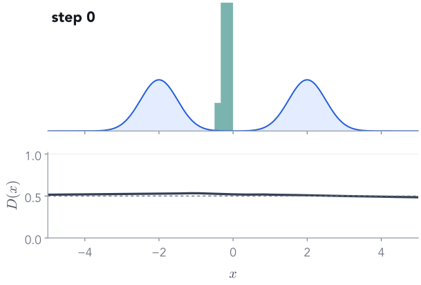
An experiment: freeze G, run only the D step

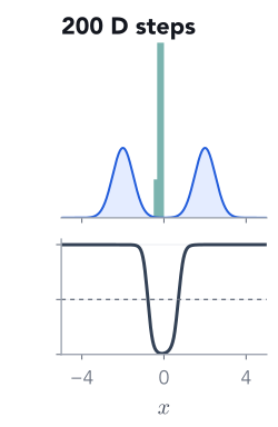
D learns to say "fake" exactly where the fakes are

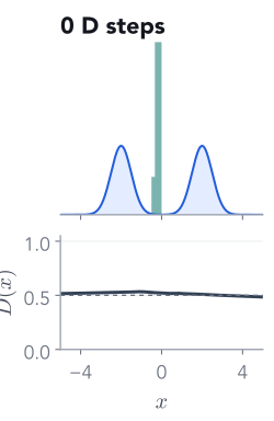
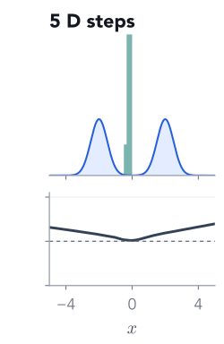
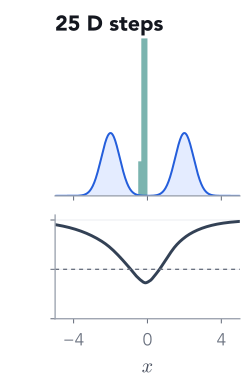
Q. G's fakes sit in one spike near 0 and never move. What should D's curve turn into?

After 200 D steps: $D = 0.01$ at the fakes, $1.00$ on the bumps, and also $1.00$ at $x = 4$, where there is no data at all.

Part 2 of 5

Training G through D

G never sees a real image and has no target output. Its only teacher is D: move each fake towards where D says "more real", and change G's weights so that it does.

✓Two players, one game
2Training G through D
3The minimax objective
4A GAN on MNIST
5Failures and control

Step 2 of each iteration: what would fool D?

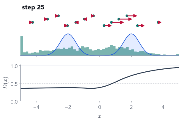
G step: push every fake uphill on $D(x)$

$$\mathcal L_G = -\log D(\cdec{G(z)})$$

The same BCE, but now the fakes are labelled 1: "make $D$ call these real".

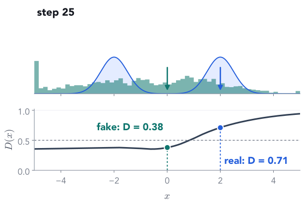
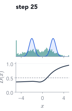
Our fake at $x = 0.0$: $D = 0.38$, so $\mathcal L_G = -\log 0.38 = 0.97$. Raising $D$ there lowers it.

Red arrows: which way $D(x)$ increases at each fake, from D's real slope at step 25.

G cannot move the fakes directly. It changes its weights $\theta$ so that its outputs move along the arrows.

Where G's gradient comes from

The chain rule runs through D

$$\frac{\partial \mathcal L_G}{\partial \theta} = \underbrace{\frac{\partial \mathcal L_G}{\partial D}}_{=\,-1/D} \cdot \underbrace{\frac{\partial D}{\partial x}}_{\text{slope of } D \text{ at the fake}} \cdot \underbrace{\frac{\partial x}{\partial \theta}}_{\text{how } \theta \text{ moves the fake}}, \qquad x = G_\theta(z)$$

$-1/D$ is always negative: raising $D$ always lowers $\mathcal L_G$. Our fake: $-1/0.38 = −2.63$.

$\partial D/\partial x$: which way is "more real" at this fake. For ours it is $0.08$: more real to the right. Uses D's weights, does not change them.

$\partial x/\partial\theta$: ordinary backprop through $G$, spreading the push over G's weights.

First two factors for our fake: $−2.63 \times 0.08 = −0.21$. Negative, so a gradient step moves it right, towards bump B.

Update G, hold D fixed

G step: lock D's weights, keep the wire

D.requires_grad_(False)                 # lock D's weights, keep the path
loss_G = bce(D(G(torch.randn(B, zdim))), ones)   # fresh fakes, no detach
opt_G.zero_grad(); loss_G.backward(); opt_G.step(); D.requires_grad_(True)

The most common GAN bug

Freezing is not detaching

Q. The wire from G to D is cut. Does G get any gradient from this loss?

Q. Now D's weights are locked but the wire is intact. Does G learn?

Detach the fake in the G step and loss_G still prints a number, but G never learns. A silent failure.

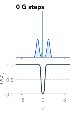
The opposite experiment: freeze D, run only the G step

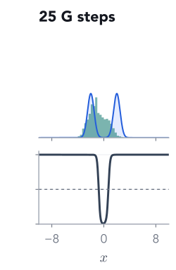
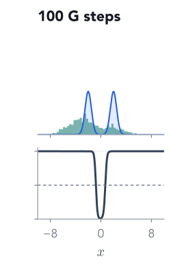
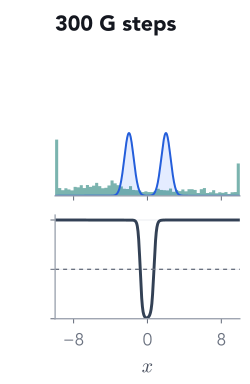
Against a judge that stops learning, G overshoots

Wider axis than before ($-10$ to $10$); fakes beyond it are piled at the edges.

Q. D (bottom) is the D from the Part 1 experiment, now frozen. Where will the fakes go?

After 300 G steps, 78% of the fakes are beyond $\pm 3$: G goes wherever D says "real", data or not. So D must keep learning, and the two steps alternate.

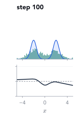
Now alternate the two steps, 3,000 times

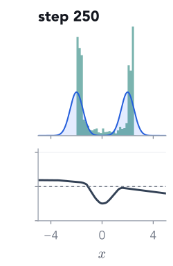
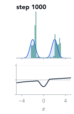
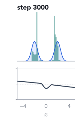
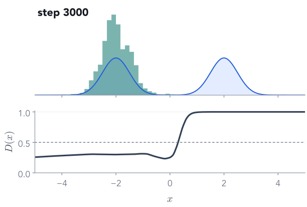
Watch the game on the toy data

By step 3,000 the fakes cover both bumps, and $D(x)$ is near 0.5 wherever the data is: it can no longer tell.

Part 3 of 5

The minimax objective

Textbooks write the whole game as one formula. Reading it slowly shows that our code trains G with a slightly different loss, and why that is a deliberate fix.

✓Two players, one game
✓Training G through D
3The minimax objective
4A GAN on MNIST
5Failures and control

The textbook formula

A two-player minimax game

$$\min_{\cdec G}\;\max_{\cdisc D}\;\; \E_{x\sim \pd}\big[\log D(x)\big] \;+\; \E_{z\sim p(z)}\big[\log\big(1 - D(G(z))\big)\big]$$

D maximises: high $D$ on real data, low $D$ on fakes. This is exactly our $-\mathcal L_D$, averaged.

G minimises: only the second term involves $G$. It wants $D(G(z))$ high.

With a perfect $D$, G's best move is $\pg = \pd$ (Goodfellow et al. 2014; derivation in the appendix). Real training, with finite networks and steps, has no such guarantee.

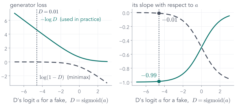
Careful: here G minimises $\log(1 - D(G(z)))$, but our code minimised $-\log D(G(z))$. Same goal. Why switch?

Two generator losses, two slopes

Differentiate both with respect to D's logit $a$

$$D = \mathrm{sigmoid}(a), \qquad \frac{dD}{da} = D\,(1-D) \qquad \text{(the logistic-regression derivative)}$$

minimax: minimise $\log(1-D)$

$$\frac{d}{da}\log(1-D) = \frac{1}{1-D}\cdot\Big(-\frac{dD}{da}\Big)$$

$$= \frac{-D(1-D)}{1-D} = \hl{-D}$$

$$D = 0.01:\quad -0.01$$

non-saturating: minimise $-\log D$

$$\frac{d}{da}\big(-\log D\big) = -\frac{1}{D}\cdot\frac{dD}{da}$$

$$= \frac{-D(1-D)}{D} = \hl{D - 1}$$

$$D = 0.01:\quad -0.99$$

Q. Early in training, which value of $D(G(z))$ is typical: near 0, near 0.5, or near 1?

Near 0: D easily rejects early fakes. There the minimax slope vanishes; the non-saturating one does not.

Why the code uses a different generator loss

Early on, the minimax loss gives G almost no signal

When D easily spots a fake ($D = 0.01$): slope $-0.01$ for $\log(1-D)$, slope $-0.99$ for $-\log D$. Same goal, a 99× stronger push.

Part 4 of 5

A GAN on MNIST

The same two steps, unchanged. Only G and D grow: small convolutional networks on 28 × 28 grey-level digits. Then back to the vote.

✓Two players, one game
✓Training G through D
✓The minimax objective
4A GAN on MNIST
5Failures and control

Only G and D grow

The MNIST generator and discriminator

G turns 100 numbers into 784 pixels; D turns 784 pixels into one logit. Each is a small CNN you already know how to build.

The complete update

One GAN iteration in code

# ---- D step: real → 1, fake → 0, G receives nothing
fake = G(torch.randn(B, zdim))
loss_D = bce_logits(D(real), ones) + bce_logits(D(fake.detach()), zeros)
opt_D.zero_grad(); loss_D.backward(); opt_D.step()

# ---- G step: fresh fakes, D's weights locked, gradient flows through D
D.requires_grad_(False)
loss_G = bce_logits(D(G(torch.randn(B, zdim))), ones)
opt_G.zero_grad(); loss_G.backward(); opt_G.step()
D.requires_grad_(True)

Exactly this function trained the 1-D GAN and the MNIST GAN. Only G and D differ.

On MNIST: the same 8 codes, through training

Watch the samples, not the loss

step 0step 50step 150step 300epoch 1epoch 3epoch 10epoch 30

Back to the vote

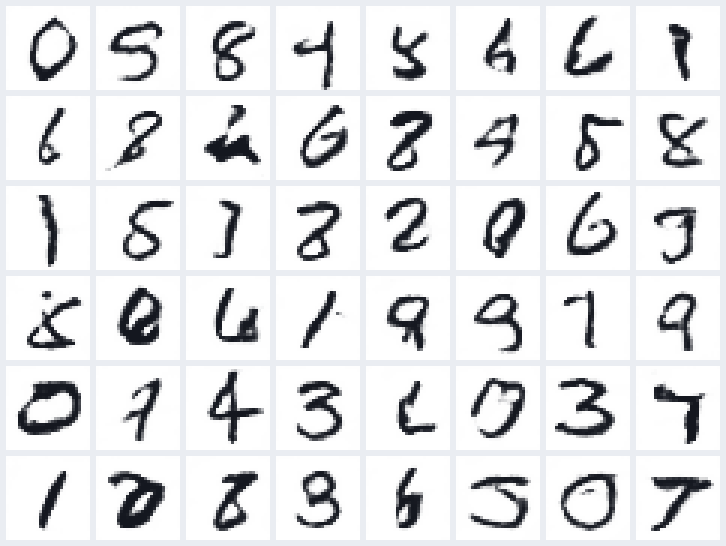
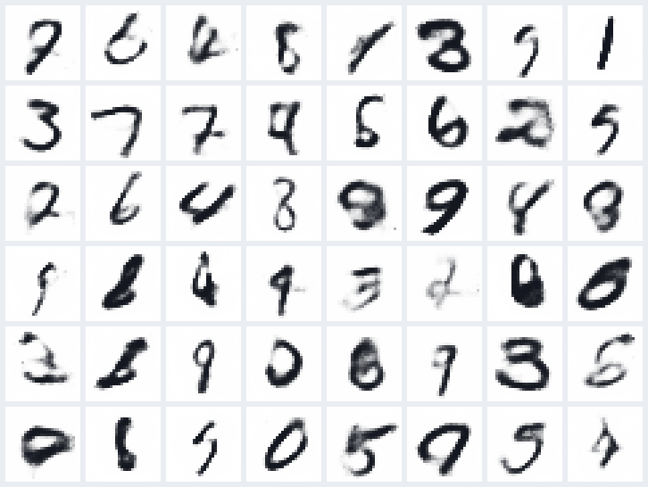
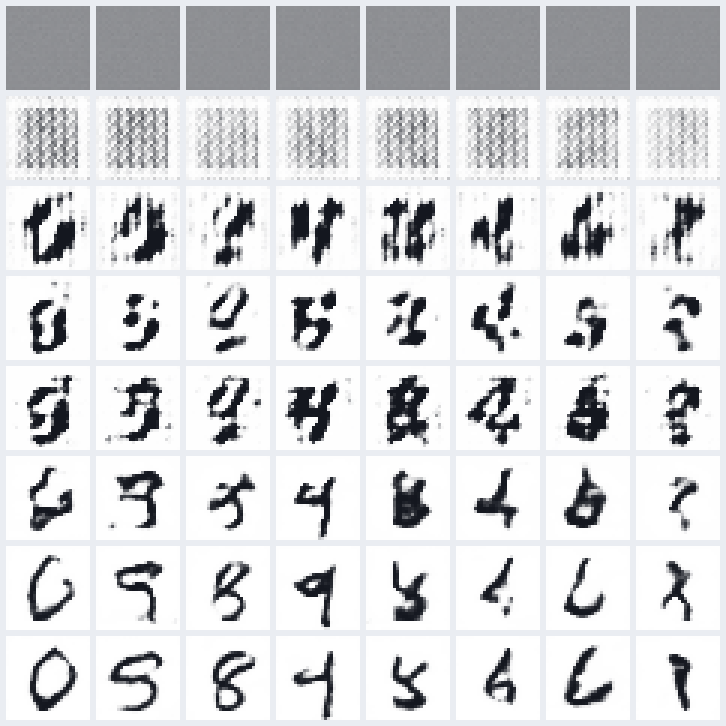
Which were real, and what did our discriminator think?

1fake · D 0.54

2real · D 0.45

3fake · D 0.55

4real · D 0.47

5real · D 0.50

6fake · D 0.50

7fake · D 0.39

8fake · D 0.42

9real · D 0.55

10fake · D 0.46

11real · D 0.48

12real · D 0.43

Q. Our trained D outputs $P(\text{real})$ for each tile. What numbers do you expect?

Every tile gets between 0.39 and 0.55. At the end of training, D can barely tell either.

Part 5 of 5

Failures and control

Every sample can look real while the model misses whole kinds of data, and the loss curves will not warn you. Then: how to ask a GAN for a particular digit.

✓Two players, one game
✓Training G through D
✓The minimax objective
✓A GAN on MNIST
5Failures and control

The classic failure

Mode collapse: perfect samples of only one kind

Same data, same training loop, but G has only 4 hidden units per layer.

After 3,000 steps: 95% of samples sit on bump A, 0% on bump B.

Every sample looks real. Bump B is never generated. Picking your favourite samples would never reveal it.

D knows: $D(+2) = 1.00$. But around bump A its curve is flat ($D \approx 0.30$, slope at most $0.04$), so no fake feels a push towards B.

Like last lecture's reverse-KL fit: commit to one mode and ignore the rest.

So how do you know it worked?

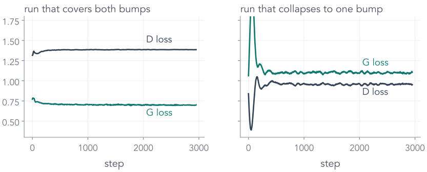
The loss curves cannot tell these two runs apart

Both curves go flat. Only the samples show that one run lost half the data. Always look at samples, from fixed $z$, across training.

Asking for a particular digit

Conditioning: tell both players what you want

Q. Give the label to G only. What stops G from ignoring it?

Nothing, unless D sees $c$ too: then a perfect 3 labelled "7" is caught as fake.

pix2pix (Isola et al. 2017) uses a whole sketch as the condition $c$, with an extra L1 term to the target photo.

Wrap-up

One GAN iteration, in four sentences

D step: binary cross-entropy, real → 1, fake → 0, with the fake detached so G gets nothing.
G step: fresh fakes labelled 1; D's weights locked, but the gradient flows through D's input into G.
Loss: minimise $-\log D(G(z))$, not $\log(1 - D(G(z)))$: same goal, no vanishing slope early on.
Judge by samples from fixed $z$, not by the losses, and look for missing modes.

✓Two players, one game
✓Training G through D
✓The minimax objective
✓A GAN on MNIST
✓Failures and control

Before you leave

Three exit questions

In the G step, why do we lock D with requires_grad_(False) instead of detaching the fake? G's gradient is $-\frac{1}{D}\cdot\frac{\partial D}{\partial x}\cdot\frac{\partial x}{\partial\theta}$: it must pass through D's input. Detaching cuts that path and G learns nothing; locking only stops D's weights from changing.
Why does the code train G on $-\log D(G(z))$ rather than minimising $\log(1 - D(G(z)))$? Early on $D(G(z)) \approx 0$. With respect to D's logit the minimax slope is $-D \approx 0$; the non-saturating slope is $D - 1 \approx -1$. Same fixed point, a push that does not vanish.
Two toy GANs both end with flat, similar losses. How would you find out that one of them has collapsed? Look at its samples from fixed $z$ next to the data: 95% on bump A and 0% on bump B. Each sample looks real; the missing bump only shows in the distribution.

Appendix

Derivations for reference

The optimal discriminator, and why a perfect D turns the game into minimising the Jensen–Shannon divergence.

Appendix A · for a fixed G

The optimal discriminator

the objective $V(D) = \displaystyle\int \Big[\pd(x)\log D(x) + \pg(x)\log\big(1-D(x)\big)\Big]\,dx$ one $x$ at a time $f(y) = a\log y + b\log(1-y), \quad y = D(x),\; a = \pd(x),\; b = \pg(x)$ set the slope to 0 $f'(y) = \dfrac{a}{y} - \dfrac{b}{1-y} = 0 \;\;\Rightarrow\;\; a(1-y) = b\,y \;\;\Rightarrow\;\; y = \dfrac{a}{a+b}$ so $D^*(x) = \dfrac{\pd(x)}{\pd(x) + \pg(x)}$

Where G puts no mass, $D^* = 1$; where $\pg = \pd$, $D^* = \tfrac12$. Our collapsed toy run never generates bump B, and its learned D there is $1.00$.

Appendix B · plug $D^*$ back in

With a perfect D, G minimises the Jensen–Shannon divergence

substitute $V(D^*, G) = \E_{\pd}\Big[\log\dfrac{\pd}{\pd + \pg}\Big] + \E_{\pg}\Big[\log\dfrac{\pg}{\pd + \pg}\Big]$ the average $m$ $m = \tfrac12(\pd + \pg), \qquad \dfrac{\pd}{\pd + \pg} = \dfrac12\cdot\dfrac{\pd}{m}$ split the logs $= -\log 2 + \E_{\pd}\Big[\log\dfrac{\pd}{m}\Big] \;-\; \log 2 + \E_{\pg}\Big[\log\dfrac{\pg}{m}\Big]$ two KLs $= -\log 4 + \KL(\pd \,\|\, m) + \KL(\pg \,\|\, m) = -\log 4 + 2\,\JS(\pd \,\|\, \pg)$

$\JS \ge 0$, and $\JS = 0$ only when $\pg = \pd$: the best G reaches $V = -\log 4 \approx −1.386$, with $D^* = \tfrac12$ everywhere. Idealised: real D and G are finite networks trained for finitely many steps.

Goodfellow et al., Generative Adversarial Nets, NeurIPS 2014, Theorem 1.

Where to go next

Goodfellow et al., Generative Adversarial Nets, arXiv 1406.2661: the game, $D^*$ and the non-saturating loss
Radford, Metz & Chintala, DCGAN, arXiv 1511.06434: the convolutional recipe our small MNIST G and D loosely follow
Lilian Weng, From GAN to WGAN (lilianweng.github.io): why GAN training is hard, and what WGAN changes
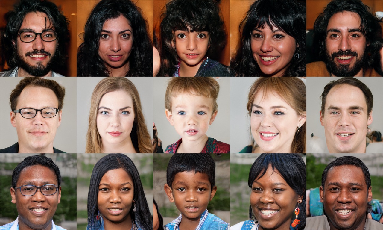
Isola et al., pix2pix, arXiv 1611.07004 · Karras et al., StyleGAN, arXiv 1812.04948
This lecture's code: scripts/train_models.py (both GANs, gan_step) and scripts/make_figures.py (every number on the slides)