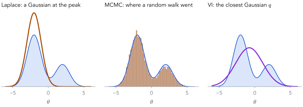
KL divergence and variational inferenceA coin, two Gaussians and two mixtures, following the PML course
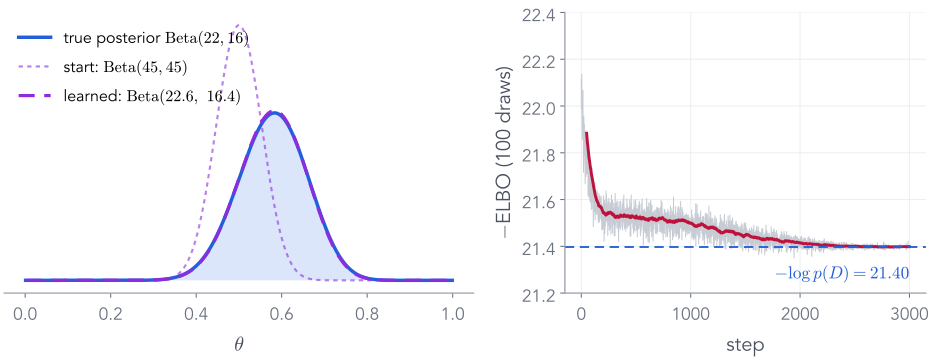
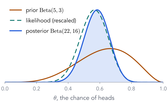
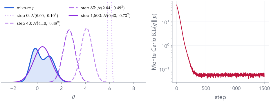
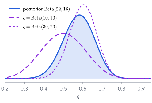
Left: a simple $\mathrm{Beta}$ guess (purple) is trained until it sits on the coin's posterior (blue). Right: the training loss settles at exactly $-\log p(D)$. By the end of today, every part of that picture will mean something precise.
A reminder: Bayes' rule, and why its denominator is hard
Everything today is about one quantity we want, the posterior, and one we cannot compute, the evidence. Ten minutes on what they are, on examples you have seen, before we learn to get around the second.
1Recap: Bayes, and why the evidence is hard
2KL divergence: how far is q from p?
3Fitting q by gradient descent
4No formula for KL? Monte Carlo
5Gradients through samples
6The ELBO
7VI for the coin
8Linear regression: correlated weights
9Neural networks and the VAE
Bayes' rule, the way the PML course began
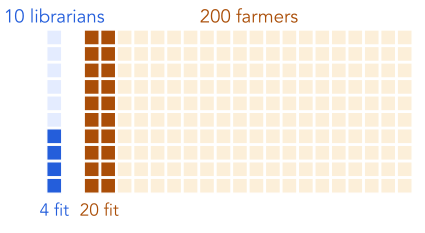
Steve is meek and orderly. Librarian or farmer?
librarian
farmer
prior: out of 210 people
10
200
likelihood: fits the description
40%
10%
people who fit
4
20
posterior: share of those who fit
4/24 = 0.167
0.833
The description fits librarians four times better, yet Steve is five times likelier a farmer. The prior matters.
▶ Notebook N1 · from PML Lecture 2 (Bayes for ML)
Bayes' rule for machine learning
"Job" becomes the parameters $\theta$; "description" becomes the data $D$
$\log p(D) = −21.397$from the formula; a 1-D grid over $\theta$ agrees: −21.397
$B(a, b) = \int_0^1 \theta^{a-1}(1-\theta)^{b-1}d\theta$ is the Beta function. The product of prior and likelihood is again a Beta shape, so the integral is known. A prior with this property is called conjugate.
Remember $-21.40$: at the end of the lecture, variational inference will recover it without the formula.
The denominator, for linear regression ▶ N1
Linear regression also has a formula for the evidence
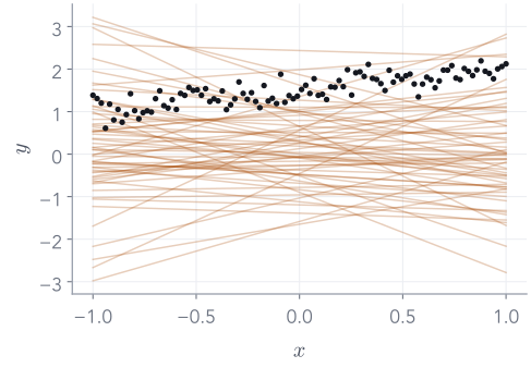
100 points from $y = 1.5 + 0.5\,x + \text{noise}$ (noise sd 0.2). Prior on the two weights: $\theta \sim \N(0, I)$.
The evidence averages the likelihood over every line the prior allows (60 of them drawn, in orange):
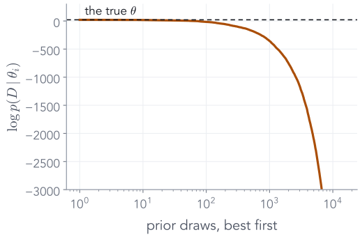
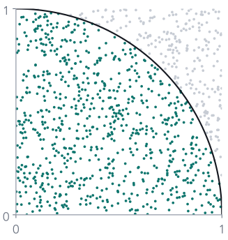
The best 10 of the 15,000 draws carry 95% of the average. The typical draw has $\log p(D\mid\theta_i)$ of about −3,497, against 20.7 at the true $\theta$.
Two weights, and sampling the prior already wastes almost every draw. With millions of weights it is hopeless.
When there is no formula at all
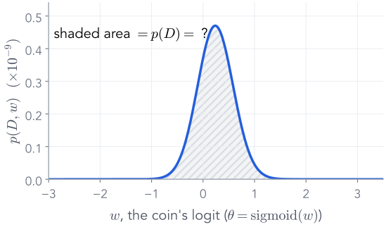
Change the prior a little, and the integral has no closed form
The same coin, but put a Normal prior on its logit: $\theta = \mathrm{sigmoid}(w)$, $w \sim \N(0, 1)$.
G1Which $q$ is closer?the KL divergence, by formula · Part 2
G2Find the closest $q$gradient descent on its parameters · Part 3
G3No formula for the KL?Monte Carlo · Part 4
G4Gradients through samplesthe reparameterisation trick · Part 5
G5How many samples?the estimate's noise · Part 4
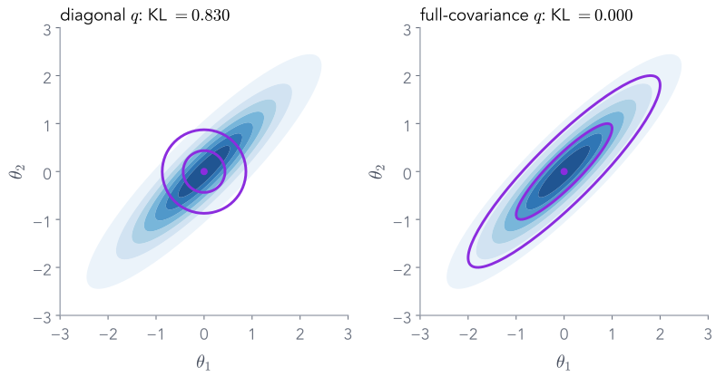
G6Diagonal or full covariance?Parts 3 and 8
Then the ELBO (Part 6) removes the one thing we cannot compute, and the coin (Part 7) puts it all together.
PML Lecture 23 at 3:06–4:38 · goals G1–G6 from cell 0 of the PML notebook variational-inference.ipynb
Part 2 of 9 · goal G1
KL divergence: how far is one distribution from another?
We will build it from a small problem, one step at a time, until the formula is the only sensible answer. Then we use it on Gaussians and on a mixture.
✓Recap: Bayes, and why the evidence is hard
2KL divergence: how far is q from p?
3Fitting q by gradient descent
4No formula for KL? Monte Carlo
5Gradients through samples
6The ELBO
7VI for the coin
8Linear regression: correlated weights
9Neural networks and the VAE
Start from a problem
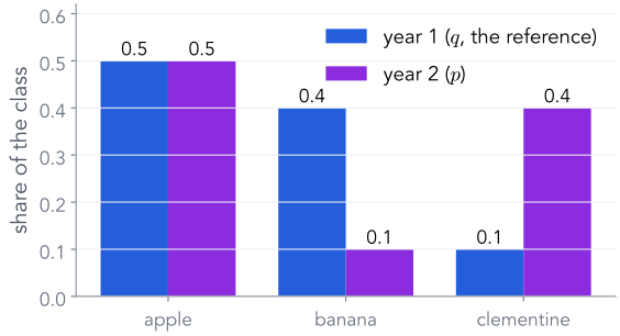
A class's favourite fruit, two years running
Year 1 is our reference, $q$: 50% apple, 40% banana, 10% clementine. Year 2, $p$: 50%, 10%, 40%.
We want one number for how much year 2 differs, relative to year 1.
"Relative to" matters. Clementine rose from 10% to 40%: a big surprise if you expected year 1. Banana fell from 40% to 10%. The two changes need not count the same.
So the number need not be symmetric. Where would you start?
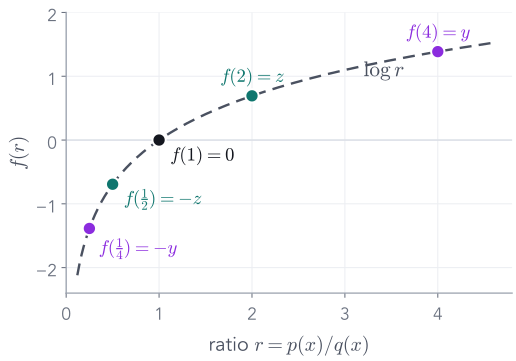
Step 1: compare by ratios. Step 2: take the log
Ratios say "how many times more"; logs make up and down cancel
apple
banana
clementine
$p/q$
1
$\tfrac14$
4
$\log(p/q)$
0
$-1.386$
$1.386$
The plain average of the ratios is 1.75: pulled up by the 4, while the $\tfrac14$ barely registers.
We want $f(1) = 0$ (no change), and $f(4) = -f(\tfrac14)$ (four times up undoes four times down). The function that does this is the log.
After the log, a fourfold rise and a fourfold fall are $\pm1.386$: equal and opposite.
Step 3: weight by what is common ▶ N2
Average the log-ratio, weighting each fruit by how common it is in $p$
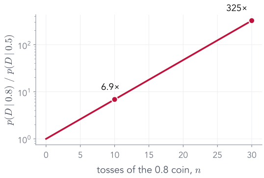
If the coin really is 0.8, each toss adds on average 0.193 nats of evidence for it. After $n$ tosses it is about $e^{n\,\KL}$ times likelier than the fair coin: 6.9× after 10, 325× after 30.
Not symmetric, and not abstract: KL is the rate at which data separate two hypotheses.
Goal G1, the PML notebook's first example ▶ N2
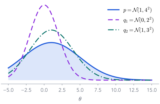
Which $q$ is closer to $p = \N(1, 4^2)$?
$q_1 = \N(0, 2^2)$: wrong centre, too narrow. $q_2 = \N(1, 3^2)$: right centre, a bit narrow. Vote.
# torch/distributions/kl.py: here p is the FIRST argument (our q)@register_kl(Normal, Normal)def_kl_normal_normal(p, q): var_ratio = (p.scale / q.scale).pow(2) t1 = ((p.loc - q.loc) / q.scale).pow(2)return0.5 * (var_ratio + t1 - 1 - var_ratio.log())
Same formula, rearranged: var_ratio is $\sigma_q^2/\sigma_p^2$ and t1 is the squared shift in units of $\sigma_p$.
With $p = \N(0, 1)$ it becomes $\tfrac12\big(\sigma^2 + \mu^2 - 1 - \log\sigma^2\big)$: the KL term of every VAE.
When both distributions are Gaussian, the KL is a formula, and torch has it. What if they are not?
PML Lecture 23, "Exercise" frame 4, 22:59–28:48
Which direction? Back to the two-bump posterior ▶ N2
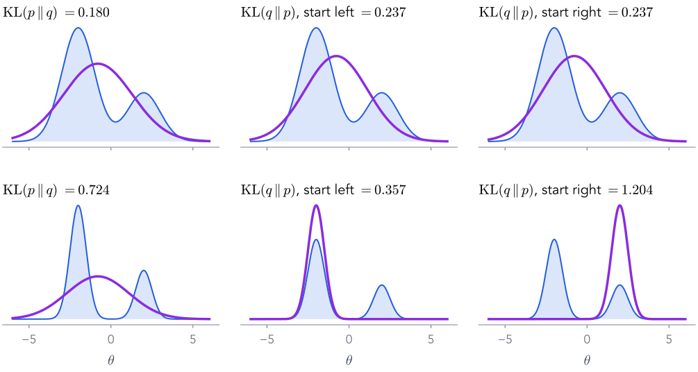
$\KL(p\|q)$ covers both bumps; $\KL(q\|p)$ picks one
Top, bumps of width 1 (Part 1's mixture): they overlap, and every fit is broad.
Bottom, bumps of width 0.5. $\KL(p\|q)$ averages under $p$: $q$ must cover both (0.724).
$\KL(q\|p)$ averages under $q$: mass in the gap costs a lot, so $q$ sits on one bump. Start left: 0.357. Start right: 1.204, a local optimum.
VI minimises $\KL(q\|p)$, because we can draw from $q$, not from the posterior. Expect $q$ to be too narrow.
Jia-Bin Huang, 4:39–5:25 · mixture from the PML Laplace notebook
Try it
Press play: the same $q$, fitted with the KL each way
$\KL(p\,\|\,q)$ = — · mean —, sd —$\KL(q\,\|\,p)$ = — · mean —, sd —
bumps$\KL(q\|p)$ startsstep 0
Same start, same optimiser; only the direction of the KL differs. Then restart the right panel from the right.
Part 3 of 9 · goal G2
Given $p$, find the closest $q$ by gradient descent
KL gives every candidate $q$ a score. Now treat the score as a loss, and let an optimiser move $q$'s parameters. The target stays simple for now, $p = \N(1, 4^2)$, so we can check every answer.
✓Recap: Bayes, and why the evidence is hard
✓KL divergence: how far is q from p?
3Fitting q by gradient descent
4No formula for KL? Monte Carlo
5Gradients through samples
6The ELBO
7VI for the coin
8Linear regression: correlated weights
9Neural networks and the VAE
First attempt: try a few candidates ▶ N3
Score a grid of $(\text{loc}, \text{scale})$ pairs against $p = \N(1, 4^2)$
$\KL(q\,\|\,p)$
scale 1
scale 2
scale 4
loc 0
0.949
0.349
0.031
loc 1
0.918
0.318
0.000
for loc in [0., 1.]:for scale in [1., 2., 4.]: print(loc, scale, dist.kl_divergence(dist.Normal(loc, scale), p))
The grid found $p$ itself, only because we put it on the grid. With more parameters a grid is hopeless.
PML notebook, cells 14–15 · PML Lecture 23 at 10:40–12:13
Then gradient descent ▶ N3
Make loc and scale parameters, and minimise the KL with Adam
A trainable $q$. The scale must stay positive, so we learn a raw number and pass it through $\mathrm{softplus}(r) = \log(1 + e^{r}) > 0$.
Start far away: $q = \N(4, 0.5^2)$, the PML notebook's starting point.
The loop. Every step: compute the KL, backpropagate to loc and raw_scale, take a step. Nothing here is specific to Gaussians except the formula inside kl_divergence.
The loss is a KL; the parameters are a distribution's. Otherwise this is any training loop you have written.
PML notebook, cells 16–17 · PML Lecture 23 at 12:13–14:33
Watch it ▶ N3
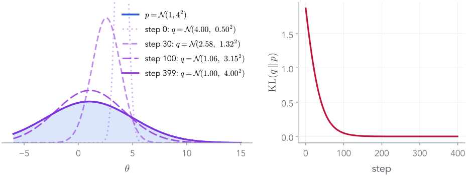
Press play: $q$ becomes $p$
step 0 of 400
$q = \N($4.00, 0.50$^2)$
$\KL(q\,\|\,p) = $ 1.869
$p = \N(1, 4^2)$$q$KL, by step
From $\N(4, 0.5^2)$ to $\N(1.00, 4.00^2)$: the KL falls from 1.87 to zero.
What the optimiser did
The centre moves first, then the width catches up
step
loc
scale
KL
0
4.00
0.50
1.869
10
3.50
0.73
1.418
30
2.58
1.32
0.740
100
1.06
3.15
0.049
399
1.00
4.00
0.000
Gradient descent found $p$ without being told where it was, only how far away each guess was.
When there is no formula for the KL, estimate it by sampling
Real posteriors are not Gaussian, so the KL between our $q$ and the target has no formula. But a KL is an average under $q$, and we can draw from $q$ as often as we like.
✓Recap: Bayes, and why the evidence is hard
✓KL divergence: how far is q from p?
✓Fitting q by gradient descent
4No formula for KL? Monte Carlo
5Gradients through samples
6The ELBO
7VI for the coin
8Linear regression: correlated weights
9Neural networks and the VAE
A target from another family ▶ N4
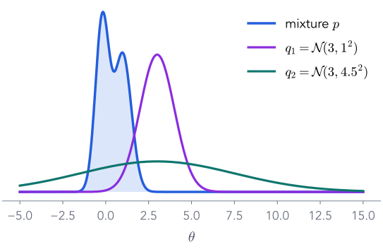
Two bumps, and two Gaussian candidates. Which is closer?
torch has no formula between a Gaussian and a mixture
p_s = MixtureSameFamily(Categorical(torch.tensor([0.5, 0.5])), Normal(torch.tensor([-0.2, 1.0]), torch.tensor([0.4, 0.5])))q_1 = dist.Normal(3., 1.)dist.kl_divergence(q_1, p_s)# NotImplementedError: No KL(p || q) is implemented for p type Normal# and q type MixtureSameFamily
The KL of a Gaussian from a mixture of Gaussians is an integral of $\log$ of a sum. It has no closed form. Neither will the KL to a real posterior.
We cannot integrate it. Can we average it?
PML notebook, cell 29 · PML Lecture 23 at 29:36–30:24
Monte Carlo, the general form
Any average under $p$ can be estimated from draws of $p$
defkl_via_sampling(q, p, n_samples=100_000): sample_set = q.sample([n_samples]) # from the FIRST argumentreturn torch.mean(q.log_prob(sample_set) - p.log_prob(sample_set))
exact
sampling
$\KL(q_1\,\|\,q_2)$, two Gaussians
1.0288
1.0276
$\KL(q_1\,\|\,p)$, mixture
none
9.45
$\KL(q_2\,\|\,p)$, mixture
none
45.02
Check it where we know the answer, then use it where we do not: $q_1$ wins, by a factor of five.
PML notebook, cells 30–35 · PML Lecture 23 at 30:24–34:39 · Lecture 24 at 6:18–8:40
Goal G5: how many samples? ▶ N4
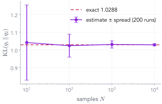
Unbiased, but the noise shrinks only like $1/\sqrt{N}$
Run kl_via_sampling 200 times for each $N$, on $\KL(q_1\,\|\,q_2)$ where the answer is 1.0288.
$N$
10
100
1,000
10,000
spread
0.212
0.065
0.021
0.007
The average is right at every $N$ (unbiased). Each 100× more samples buys 10× less noise.
For training we only need an unbiased estimate: a noisy loss gives a noisy, but correct on average, gradient.
Gradients through random samples: the reparameterisation trick
We can estimate the KL to a mixture by sampling from $q$. To minimise it we need its gradient with respect to $q$'s parameters, and a random draw seems to have none.
✓Recap: Bayes, and why the evidence is hard
✓KL divergence: how far is q from p?
✓Fitting q by gradient descent
✓No formula for KL? Monte Carlo
5Gradients through samples
6The ELBO
7VI for the coin
8Linear regression: correlated weights
9Neural networks and the VAE
The original formulation, as a computational graph
The loss depends on loc and scale only through a random draw
Backpropagation needs a derivative at every node. "Draw a sample" has none: the path is blocked.
loc = torch.tensor(2.0, requires_grad=True)scale = torch.tensor(0.5, requires_grad=True)q = dist.Normal(loc, scale)s = q.sample()s.backward()# RuntimeError: element 0 of tensors does not require grad# and does not have a grad_fn
The sample s is a plain number with no history. Any loss built from it, like kl_via_sampling, gives no gradient to loc or scale.
So we cannot yet train $q$ on the Monte Carlo KL. We need the randomness to sit somewhere else.
PML notebook, cell 39 · PML Lecture 24 at 9:27–10:15
The reparameterised formulation
Draw the noise from a fixed $\N(0, 1)$; then shift and stretch it
$$\varepsilon \sim \N(0, 1), \qquad z = \text{loc} + \text{scale}\cdot\varepsilon \quad\Longrightarrow\quad z \sim \N(\text{loc},\ \text{scale}^2)$$
✎Before the next click: what are $\partial z/\partial\,\text{loc}$ and $\partial z/\partial\,\text{scale}$?
PML notebook, cells 43–45 and 49 (reparam.002) · PML Lecture 23 at 38:53–41:33
Check the exercise in code ▶ N5
Now the draw has a gradient: $\partial z/\partial\,\text{loc} = 1$, $\partial z/\partial\,\text{scale} = \varepsilon$
torch.manual_seed(42)loc = torch.tensor(2.0, requires_grad=True)scale = torch.tensor(0.5, requires_grad=True)eps = dist.Normal(0., 1.).sample() # randomness that does not depend on loc or scalez = loc + scale * eps # the reparameterised drawz.backward()loc.grad, scale.grad, eps # 1.0000, 0.3367, 0.3367
The gradient with respect to scale is the noise that was drawn. Different draw, different gradient: noisy but unbiased.
PML notebook, cell 44 · PML Lecture 24 at 11:02–13:26
Each step: draw $\varepsilon$, form $z = \text{loc} + \text{scale}\cdot\varepsilon$, average $\log q(z) - \log p(z)$, and follow its gradient.
Part 6 of 9
The ELBO: a loss we can compute without the posterior
Parts 2–5 fitted $q$ to targets we could evaluate. The posterior is not one of them: we cannot evaluate $p(\theta\mid D)$, only $p(D\mid\theta)\,p(\theta)$. Three short algebra steps fix this.
✓Recap: Bayes, and why the evidence is hard
✓KL divergence: how far is q from p?
✓Fitting q by gradient descent
✓No formula for KL? Monte Carlo
✓Gradients through samples
6The ELBO
7VI for the coin
8Linear regression: correlated weights
9Neural networks and the VAE
The catch
The KL we want to minimise contains the posterior itself
$$= \underbrace{\E_q\big[\log p(D\mid\theta)\big]}_{\text{fit the data}} \;-\; \underbrace{\KL\big(q(\theta)\,\|\,p(\theta)\big)}_{\text{stay close to the prior}}$$
The first form is what we will code for the coin. The second is the VAE's loss, with the prior $\N(0, I)$ and Part 2's Gaussian KL.
Part 7 of 9 · worked example
Variational inference for the coin, start to finish
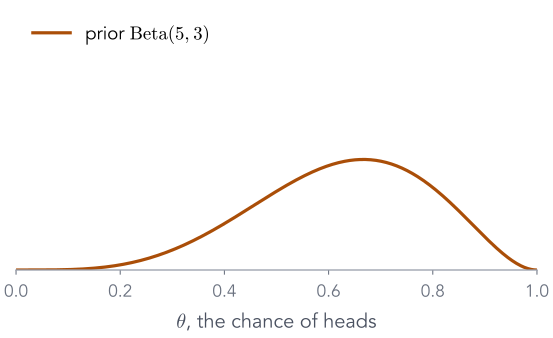
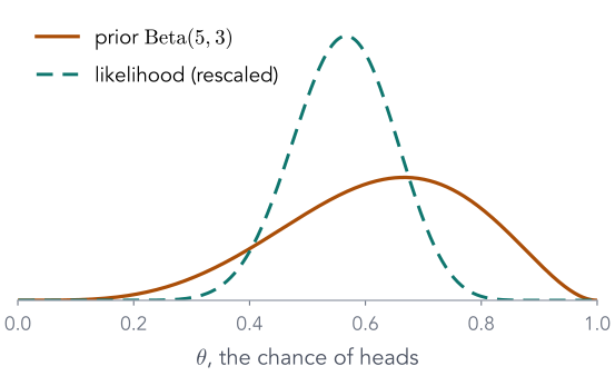
Part 1's coin: prior $\mathrm{Beta}(5, 3)$, 17 heads in 30. We know the answer, $\mathrm{Beta}(22, 16)$ and $\log p(D) = −21.40$, so we can check every step. VI will use only the joint.
✓Recap: Bayes, and why the evidence is hard
✓KL divergence: how far is q from p?
✓Fitting q by gradient descent
✓No formula for KL? Monte Carlo
✓Gradients through samples
✓The ELBO
7VI for the coin
8Linear regression: correlated weights
9Neural networks and the VAE
The model, as functions ▶ N7
All VI needs from the model is $\log p(D, \theta)$ at any $\theta$
$\theta$ lives in $[0, 1]$, so let $q$ be a $\mathrm{Beta}(\alpha, \beta)$
$q = \mathrm{Beta}(\alpha, \beta)$
Right support, two parameters, and an rsample (Part 5). Here it even contains the true posterior, so VI can be exact.
$q = \N(\mu, \sigma^2)$?
It puts mass below 0 and above 1, where $\log p(D\mid\theta)$ is undefined. The fix is to fit a Normal to $\mathrm{logit}(\theta)$ instead: automatic differentiation VI (ADVI) does this for every constrained parameter.
Parameters $\psi = (\alpha, \beta)$, both kept positive with softplus, as the scale was in Part 3.
In general the family will not contain the posterior; VI then finds the closest member. Here we get to see it hit the target.
defneg_elbo(log_joint_fn, q, n_mc_samples=100): theta = q.rsample([n_mc_samples]) # draws from q, with gradients log_q_theta = q.log_prob(theta) log_joint = log_joint_fn(theta)return -(log_joint - log_q_theta).mean()
rsample, not sample, so the loss can be differentiated with respect to $\alpha$ and $\beta$.
Evaluate $\log q$ and $\log p(D, \theta)$ at the same 100 draws.
Average, and flip the sign: optimisers minimise.
Compare Part 4's kl_via_sampling: the same code, with the joint in place of the target density.
PML notebook, cells 66–67 · PML Lecture 24 at 38:29–40:57
Score two guesses ▶ N7
A bad $q$ scores in the hundreds; the posterior scores exactly $-\log p(D)$
$q$
neg_elbo
$\mathrm{Beta}(0.1, 2)$: almost all mass near 0
239.38
PML runs: 218.88, 188.33
$\mathrm{Beta}(22, 16)$: the true posterior
21.397
$= -\log p(D)$, every run
Why exact? When $q$ is the posterior, $\log p(D, \theta) - \log q(\theta) = \log p(D)$ for every $\theta$. Each of the 100 draws gives the same number, so the estimate has no noise at all.
The first is a Monte Carlo estimate and changes from run to run. The second is the bound itself.
PML notebook, cells 68–69 (both versions of the notebook) · PML Lecture 24 at 40:57–41:46
Train it ▶ N7
From $\mathrm{Beta}(45, 45)$ to $\mathrm{Beta}(22.6, 16.4)$ in 3,000 steps
Model: prior and likelihood, as sampling statements.
Guide: our $q$, with learnable $\alpha$, $\beta$. The names must match the model's.
SVI builds neg_elbo for us. The PML run ended near $\alpha \approx 22.9$, $\beta \approx 16.7$.
Probabilistic programming languages automate exactly what we wrote by hand.
PML notebook, cells 72–77 · PML Lecture 24 at 42:32–45:41
Part 8 of 9 · worked example · goal G6
Two weights at once: VI for linear regression
The same neg_elbo, now with a 2-D $\theta$ and a 2-D Gaussian $q$. Bayesian linear regression has an exact posterior, so once more we can check the answer. If time is short, this part is homework: notebook N8.
✓Recap: Bayes, and why the evidence is hard
✓KL divergence: how far is q from p?
✓Fitting q by gradient descent
✓No formula for KL? Monte Carlo
✓Gradients through samples
✓The ELBO
✓VI for the coin
8Linear regression: correlated weights
9Neural networks and the VAE
The model, and the only new line ▶ N8
$y = 3x + 4 + \text{noise}$, and a Gaussian $q$ over (intercept, slope)
The PML notebook's data: noise of scale 5, prior $\theta\sim\N(0, I)$.
Each row of theta is one line; the likelihood scores it on every point.
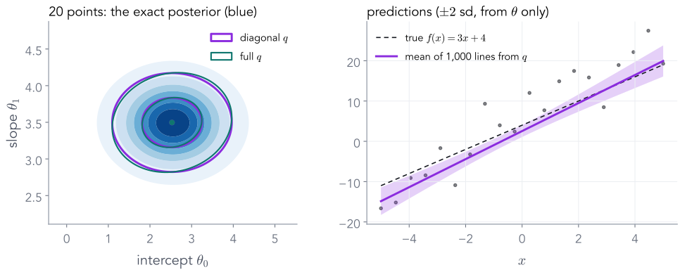
The coin's neg_elbo, unchanged. Two choices of $q$: a diagonal Gaussian (two means, two widths) or a full one, $\Sigma = LL^\top$ (one more number, the tilt).
Nothing about VI changed. Only the model's log_joint and the shape of $q$.
PML notebook, cells 78–82 · PML Lecture 24 at 56:55–57:47
20 points ▶ N8
Both $q$'s land on the exact posterior, and give a band of lines
intercept
slope
exact mean, sd
2.55, 0.745
3.49, 0.346
full $q$ by VI
2.53, 0.718
3.50, 0.340
The intercept is pulled from 4 towards the prior's 0: with 20 noisy points, the prior still matters.
PML notebook, cells 83–86 · PML Lecture 24 at 57:47–1:01:57
200 points ▶ N8
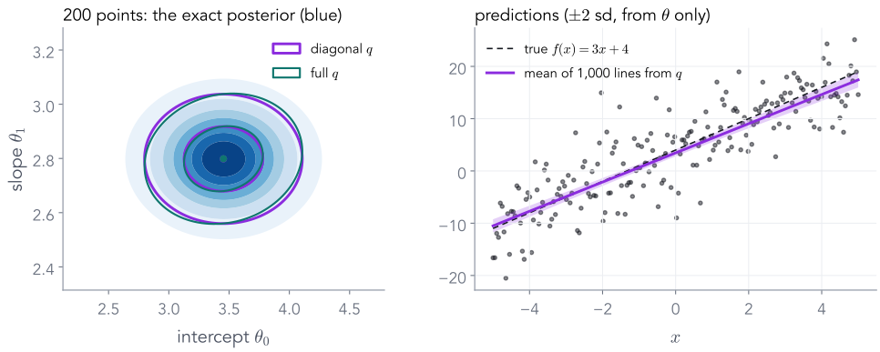
Ten times the data: the posterior, and the band, shrink
intercept
slope
exact mean, sd
3.46, 0.333
2.80, 0.121
full $q$ by VI
3.45, 0.327
2.80, 0.120
The widths fall two to three times, and the intercept moves close to 4: now the data dominate the prior.
PML notebook, cells 87–89 · PML Lecture 24 at 1:01:57–1:05:09
Part 9 of 9
Neural networks, and the VAE in one slide
What changes when $\theta$ has millions of entries, and how the same ELBO becomes the loss of a variational autoencoder.
✓Recap: Bayes, and why the evidence is hard
✓KL divergence: how far is q from p?
✓Fitting q by gradient descent
✓No formula for KL? Monte Carlo
✓Gradients through samples
✓The ELBO
✓VI for the coin
✓Linear regression: correlated weights
9Neural networks and the VAE
Millions of parameters
For a neural network, $q$ is one Gaussian per weight: mean-field
Full covariance
One mean per weight, plus a correlation for every pair. A million weights: about $5\times 10^{11}$ numbers. Impossible to store, let alone fit.
Mean-field
$q(\theta) = \prod_i \N(\theta_i\mid\mu_i, \sigma_i^2)$: two numbers per weight. Cheap, and rsample is one line, as in Part 5.
The price is Part 3's 2-D picture: no correlations, and $\KL(q\|p)$ makes each width too narrow. Bayesian neural networks trained this way tend to be over-confident.
MCMC remains the gold standard for small networks; mean-field VI is what scales.
PML Variational-Inference slides, "Neural Networks" · PML Lecture 24 at 49:02–50:39 and 52:50–56:04
Where this goes next lecture
The VAE: one posterior per image, predicted by an encoder
today
in the VAE
$\theta$, what we infer
$z$, an image's code
$D$, the data
$x$, one image
prior $p(\theta)$
$p(z) = \N(0, I)$
likelihood $p(D\mid\theta)$
the decoder $p(x\mid z)$
$q(\theta)$, one fit
$q(z\mid x) = \N\big(\mu(x), \sigma(x)^2\big)$, from an encoder
Every image has its own posterior. Fitting a $q$ per image would be slow, so a network predicts $q$'s parameters from $x$: amortised inference.
The second form from Part 6. The KL is Part 2's Gaussian formula; the expectation uses $z = \mu + \sigma\cdot\varepsilon$ from Part 5.
Nothing new is needed: a VAE is today's ELBO, with a decoder for the likelihood and an encoder for $q$.
PML Lecture 25 (VAEs) at 44:00–51:13 and 1:06:27–1:08:05
Today on one page
From Bayes' rule to a loss we can train
Bayes: posterior $\propto$ likelihood $\times$ prior→the evidence $p(D)$ is intractable→propose a simple $q$→measure closeness: $\KL(q\|p)$→fit $q$ by gradient descent→no formula? Monte Carlo→gradients through draws: rsample→the ELBO needs only the joint→the coin: VI recovers $\mathrm{Beta}(22, 16)$
$\log p(D) = \ELBO + \KL$for every $q$; the KL is $\ge 0$
$z = \mu + \sigma\cdot\varepsilon$a random draw with a gradient
Two lines to remember. The VAE lecture uses both on its first slide.
Exit questions
Five questions
Why can we not just compute $p(\theta\mid D)$ for a neural network? The evidence is an integral over millions of weights with no formula. A grid is impossible, and sampling the prior wastes almost every draw: for two weights, the best 10 of 15,000 draws already carried 95% of the estimate.
Why does VI minimise $\KL(q\|p)$ rather than $\KL(p\|q)$, and what is the price? A KL averages under its first argument, and we can draw from $q$ but not from the posterior. The price: $q$ seeks a mode and comes out too narrow.
Why does q.sample() break training, and what does rsample do instead? A sample has no gradient path. rsample draws $\varepsilon\sim\N(0, 1)$ and returns $\text{loc} + \text{scale}\cdot\varepsilon$, whose gradients are 1 and $\varepsilon$.
$\log p(D) = \ELBO(q) + \,?$ $\KL\big(q\,\|\,p(\theta\mid D)\big) \ge 0$. Since $\log p(D)$ does not depend on $q$, raising the ELBO lowers the KL, and the ELBO needs only $p(D, \theta)$.
For the coin, what does neg_elbo return at $q = \mathrm{Beta}(22, 16)$, and why is it the same on every run? 21.397 $= -\log p(D)$. At the posterior, $\log p(D, \theta) - \log q(\theta) = \log p(D)$ for every $\theta$, so every draw gives the same number.