Bias Variance Tradeoff

Author

Nipun Batra

Published

January 9, 2024

Open In Colab

import numpy as np
import matplotlib.pyplot as plt
%config InlineBackend.figure_format = 'retina'
from latexify import latexify, format_axes
from sklearn.tree import DecisionTreeRegressor
from sklearn.preprocessing import PolynomialFeatures
from sklearn.linear_model import LinearRegression
from sklearn.pipeline import make_pipeline

import pandas as pd
import ipywidgets as widgets

latexify(columns=2)

x_overall = np.linspace(0, 10, 50)
f_x = 0.2*np.sin(x_overall) + 0.2*np.cos(2*x_overall)+ 0.6*x_overall - 0.05*x_overall**2 - 0.003*x_overall**3

eps = np.random.normal(0, 1, 50)
y_overall = f_x + eps
plt.plot(x_overall, f_x, label = 'True function')
plt.scatter(x_overall, y_overall, s=10, c='r', label = 'Noisy data')
format_axes(plt.gca())
plt.legend()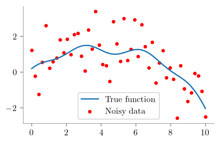

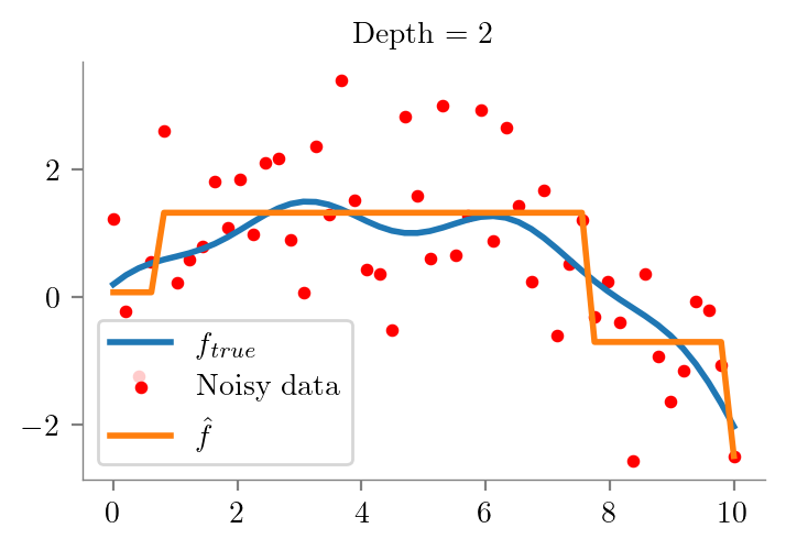
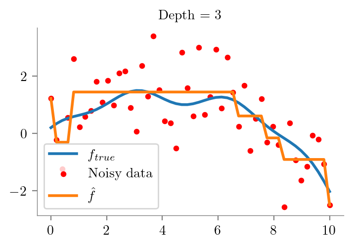
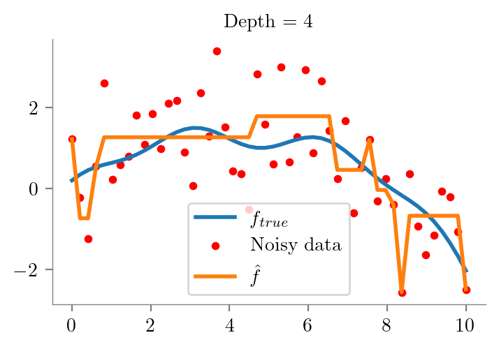
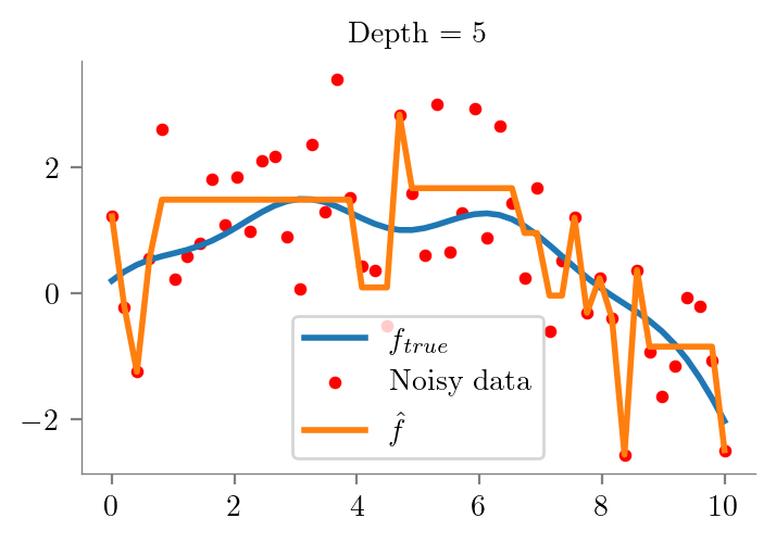
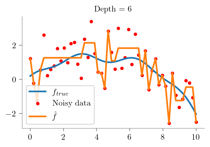
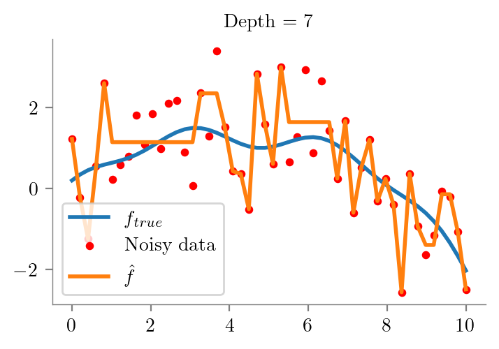
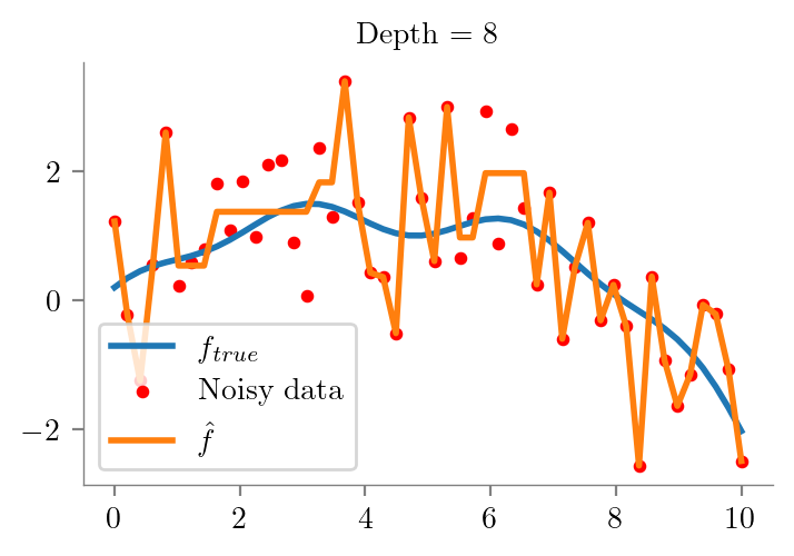
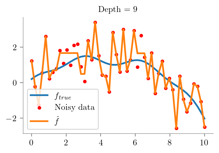
def fit_plot_tree(x, y, depth=1, extra=None):
    dt = DecisionTreeRegressor(max_depth=depth)
    dt.fit(x.reshape(-1, 1), y)
    y_pred = dt.predict(x.reshape(-1, 1))
    plt.figure()

    plt.plot(x_overall, f_x, label = r'$f_{true}$', lw=2)
    plt.scatter(x_overall, y_overall, s=10, c='r', label = 'Noisy data')
    label = r"$\hat{f}$" if not extra else fr"$\hat{{f}}_{{{extra}}}$"

    plt.plot(x, y_pred, label = label, lw=2)

    format_axes(plt.gca())
    plt.legend()
    plt.title(f"Depth = {depth}")
    return dt

for i in range(1, 10):
    fit_plot_tree(x_overall, y_overall, i)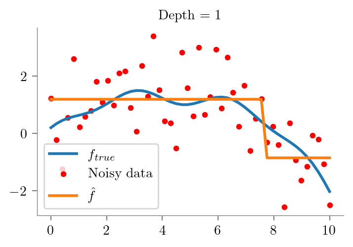

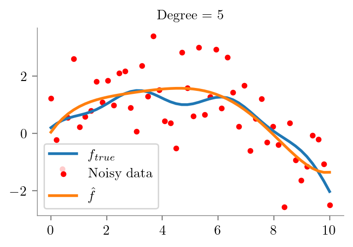
def fit_plot_polynomial(x, y, degree=1, extra=None, ax=None):
    model = make_pipeline(PolynomialFeatures(degree), LinearRegression())
    model.fit(x.reshape(-1, 1), y)
    y_pred = model.predict(x.reshape(-1, 1))
    if ax is None:
        fig, ax = plt.subplots()

    ax.plot(x_overall, f_x, label = r'$f_{true}$', lw=2)
    ax.scatter(x_overall, y_overall, s=10, c='r', label = 'Noisy data')
    label = r"$\hat{f}$" if not extra else fr"$\hat{{f}}_{{{extra}}}$"

    ax.plot(x, y_pred, label = label, lw=2)

    format_axes(ax)
    ax.legend()
    ax.set_title(f"Degree = {degree}")
    return model

fit_plot_polynomial(x_overall, y_overall, 5)

Pipeline(steps=[('polynomialfeatures', PolynomialFeatures(degree=5)),
                ('linearregression', LinearRegression())])

In a Jupyter environment, please rerun this cell to show the HTML representation or trust the notebook.
On GitHub, the HTML representation is unable to render, please try loading this page with nbviewer.org.

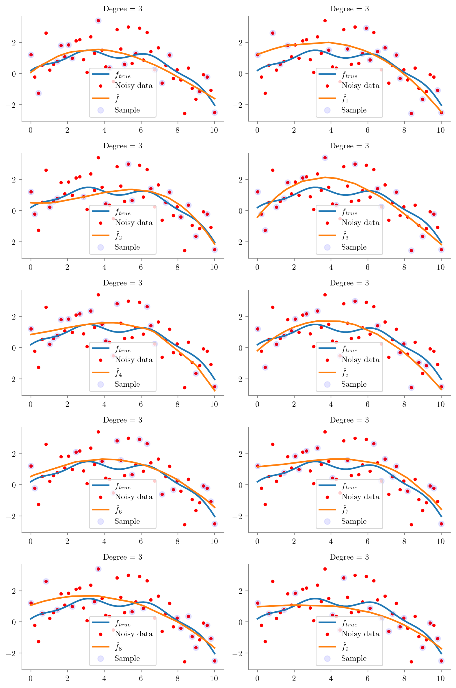
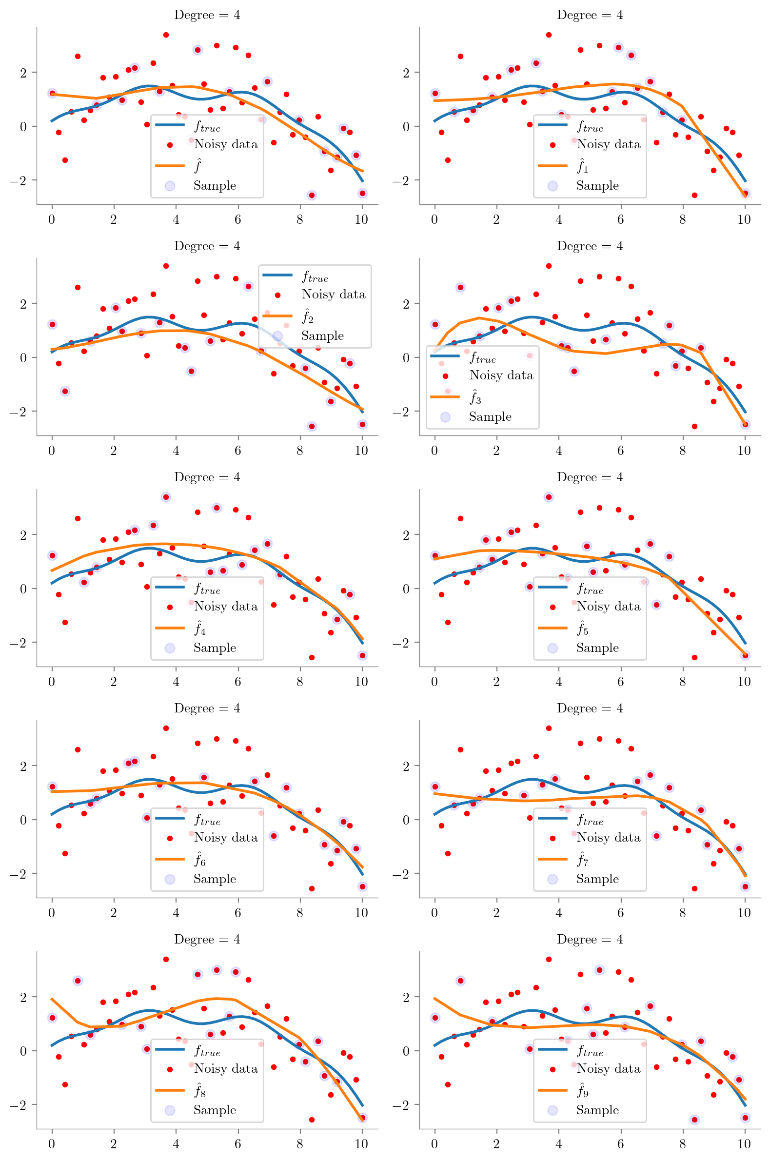
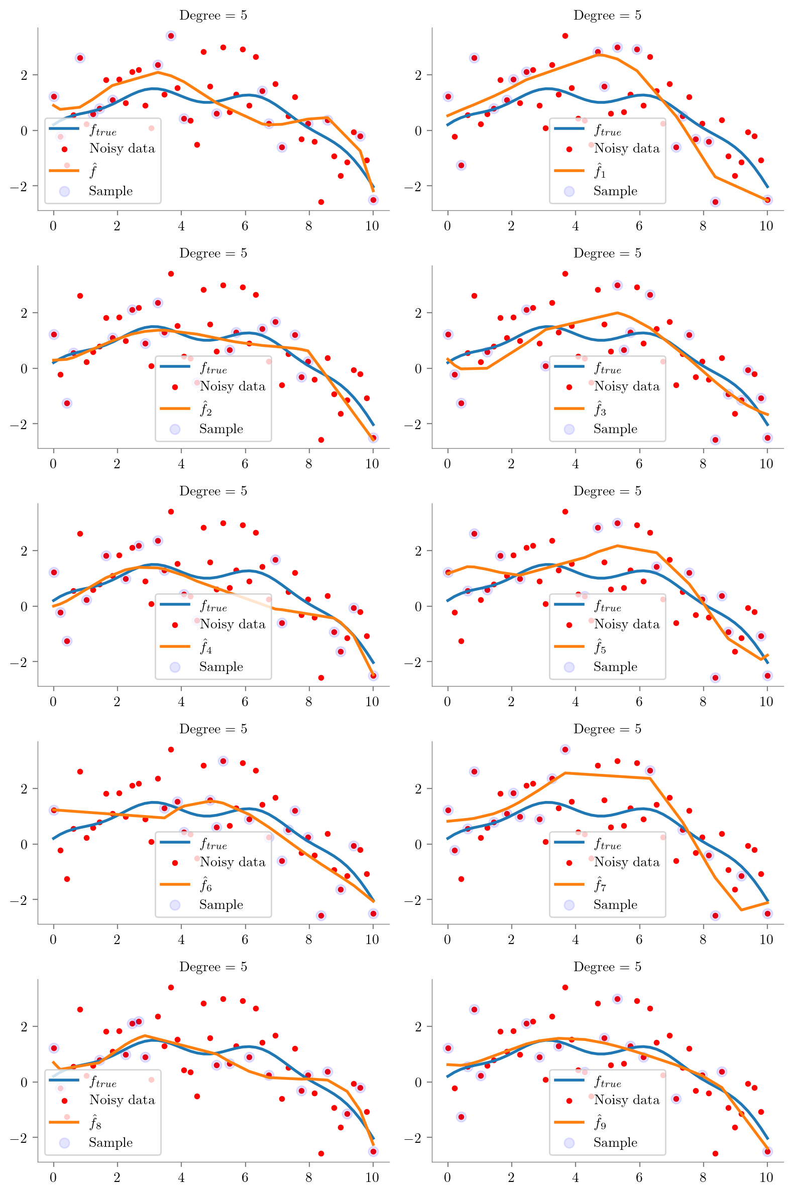
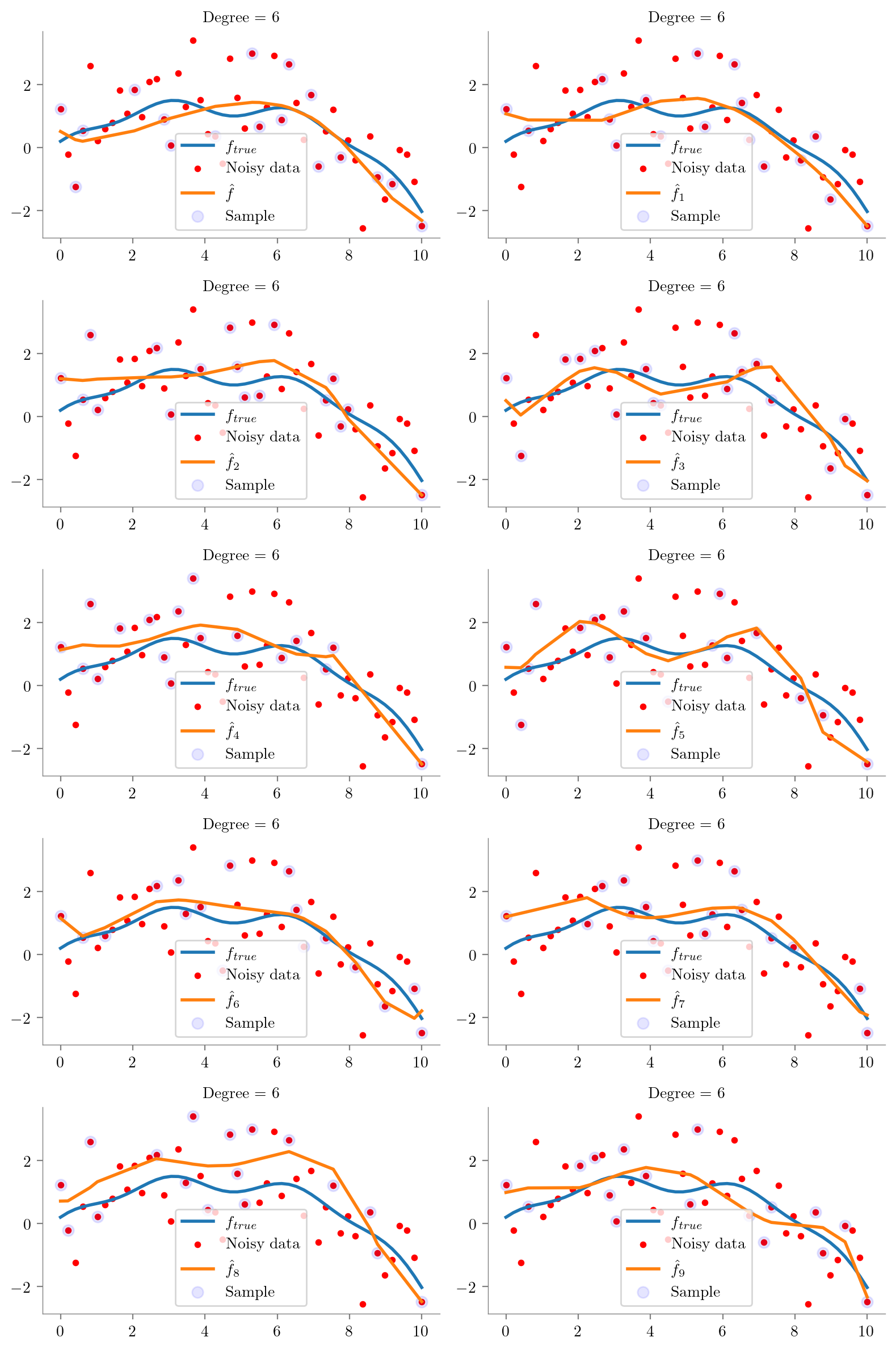
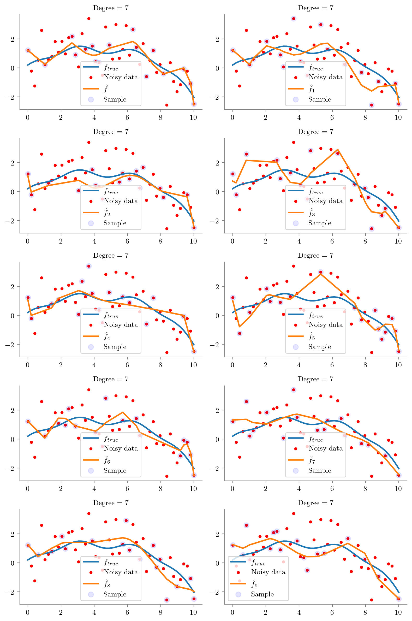
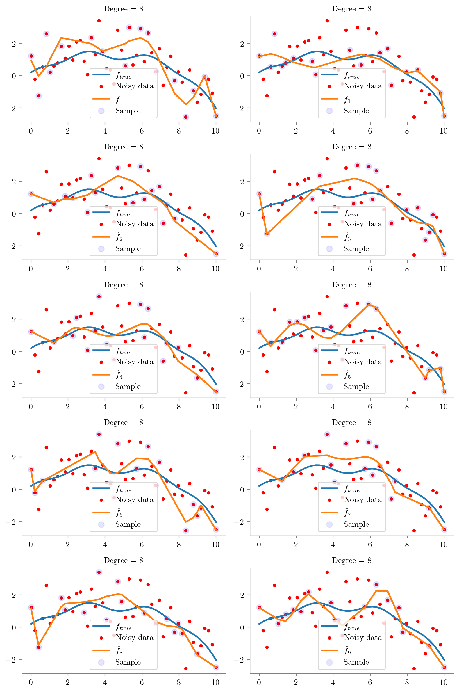
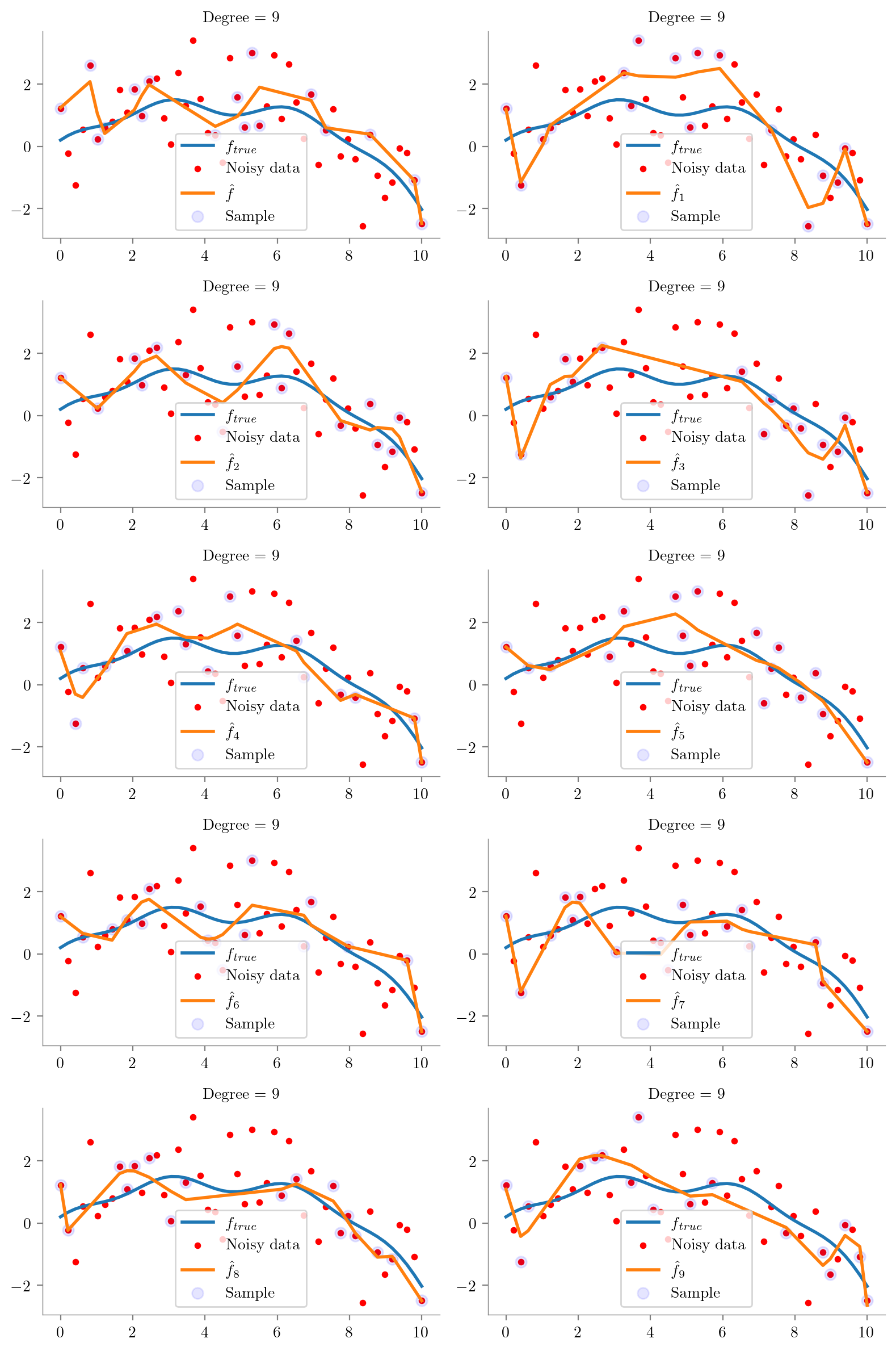
def plot_degree(degree=1):
    regs = []
    fig, axes = plt.subplots(5, 2, figsize=(8, 12), sharex=True, sharey=True)

    for i, ax in enumerate(axes.flatten()):
        idx = np.random.choice(np.arange(1, 49), 15, replace=False)
        idx = np.concatenate([[0], idx, [49]])
        idx.sort()
        x = x_overall[idx]
        y = y_overall[idx]
        regs.append(fit_plot_polynomial(x, y, degree=degree, extra=i, ax=ax))
        # remove legend
        #ax.legend().remove()
        ax.scatter(x_overall[idx], y_overall[idx], s=50, c='b', label='Sample', alpha=0.1)
        ax.legend()
    
    plt.tight_layout()
    plt.show()
    
    return regs

_ = plot_degree(5)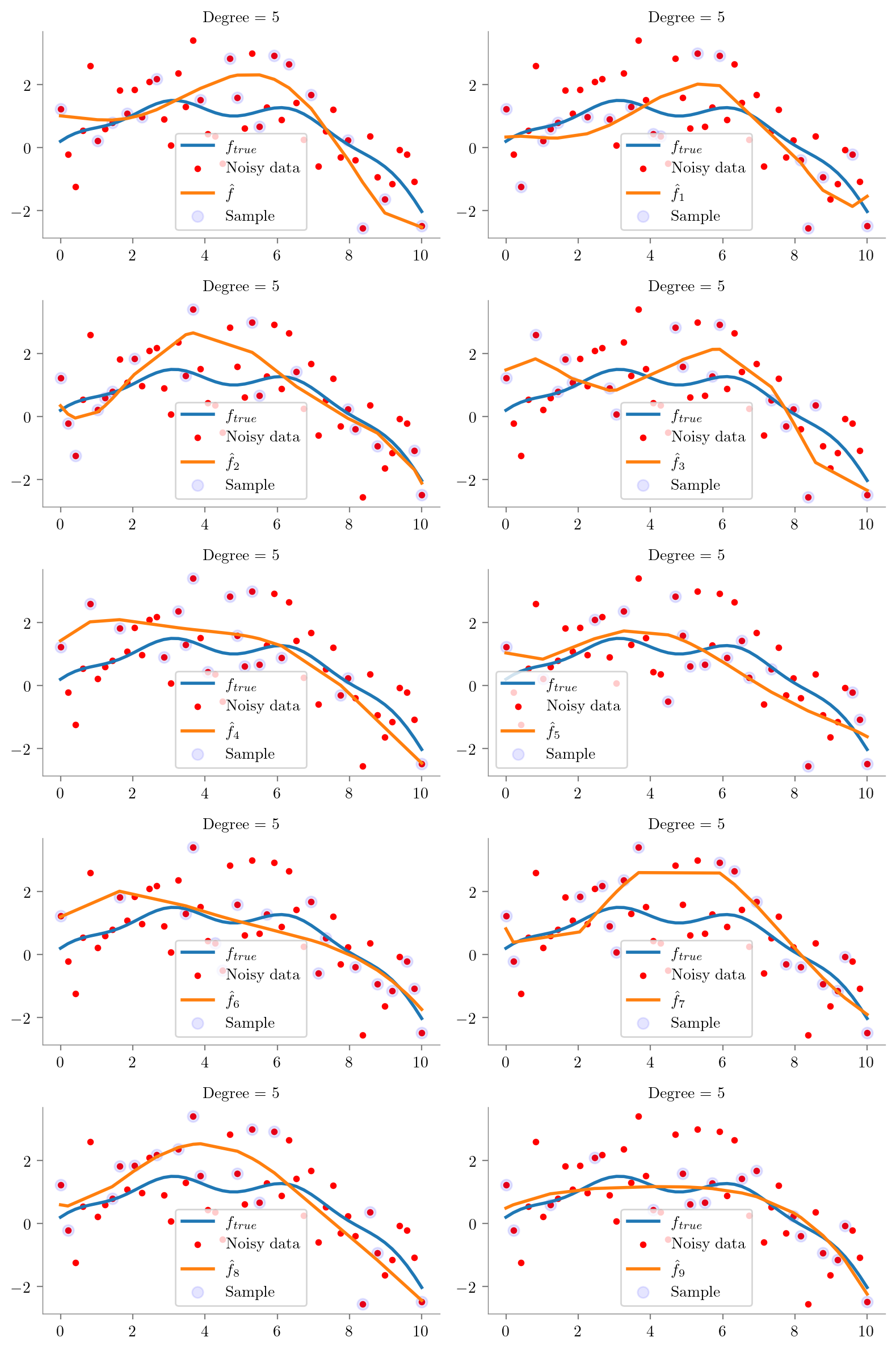

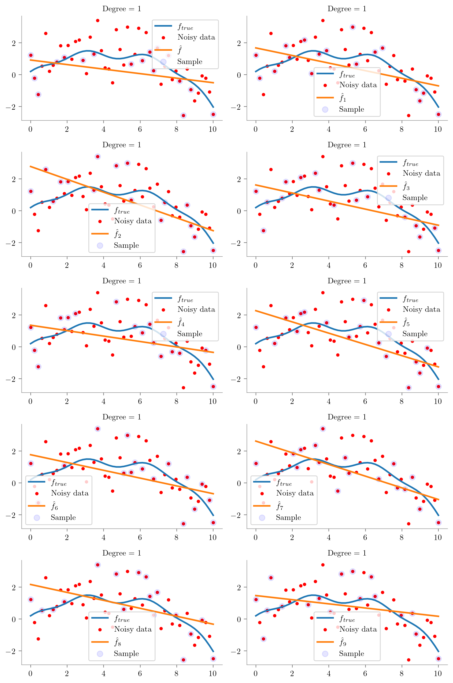
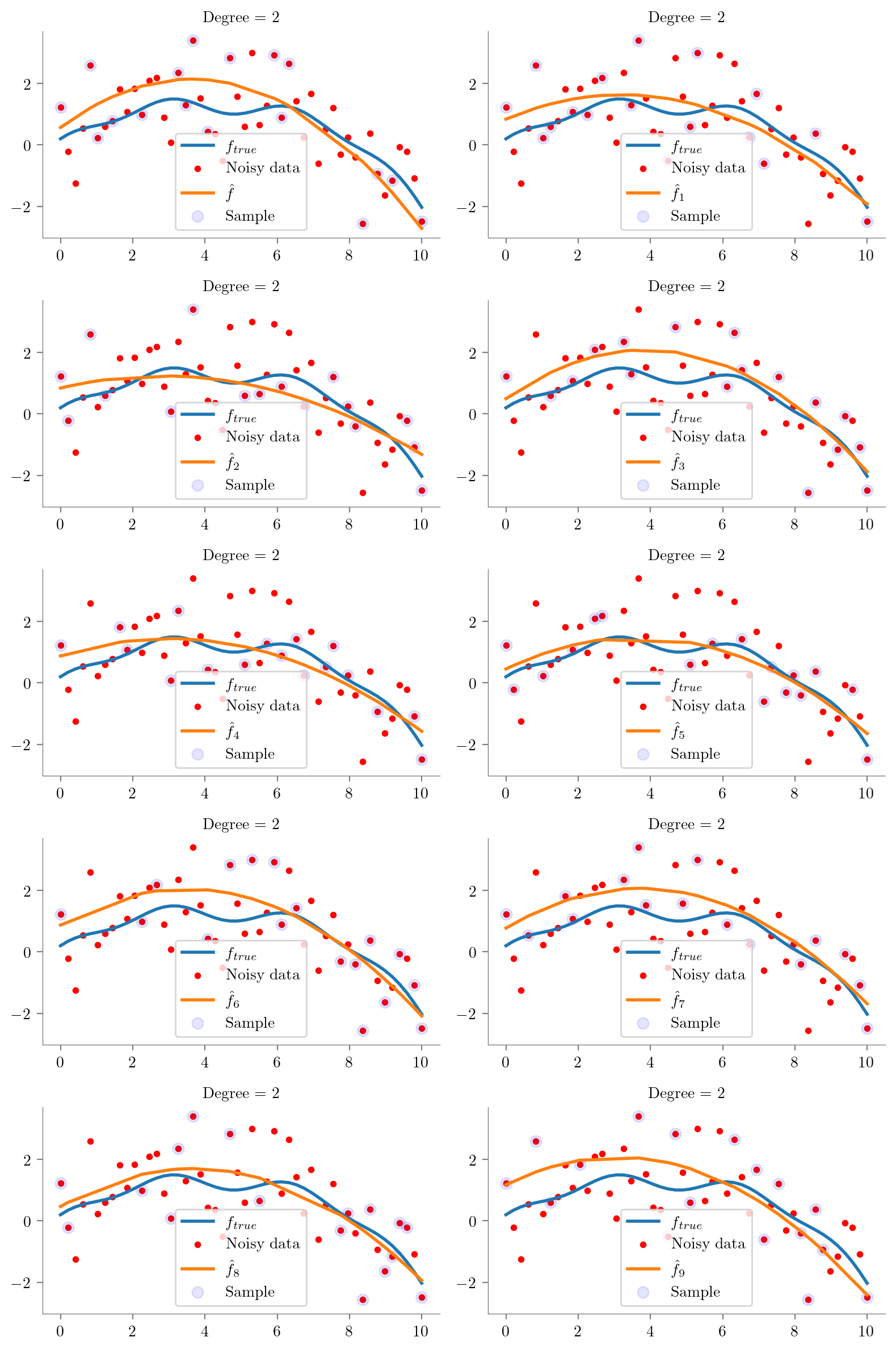
regs = {}
for i in range(0, 10):
    regs[i] = plot_degree(i)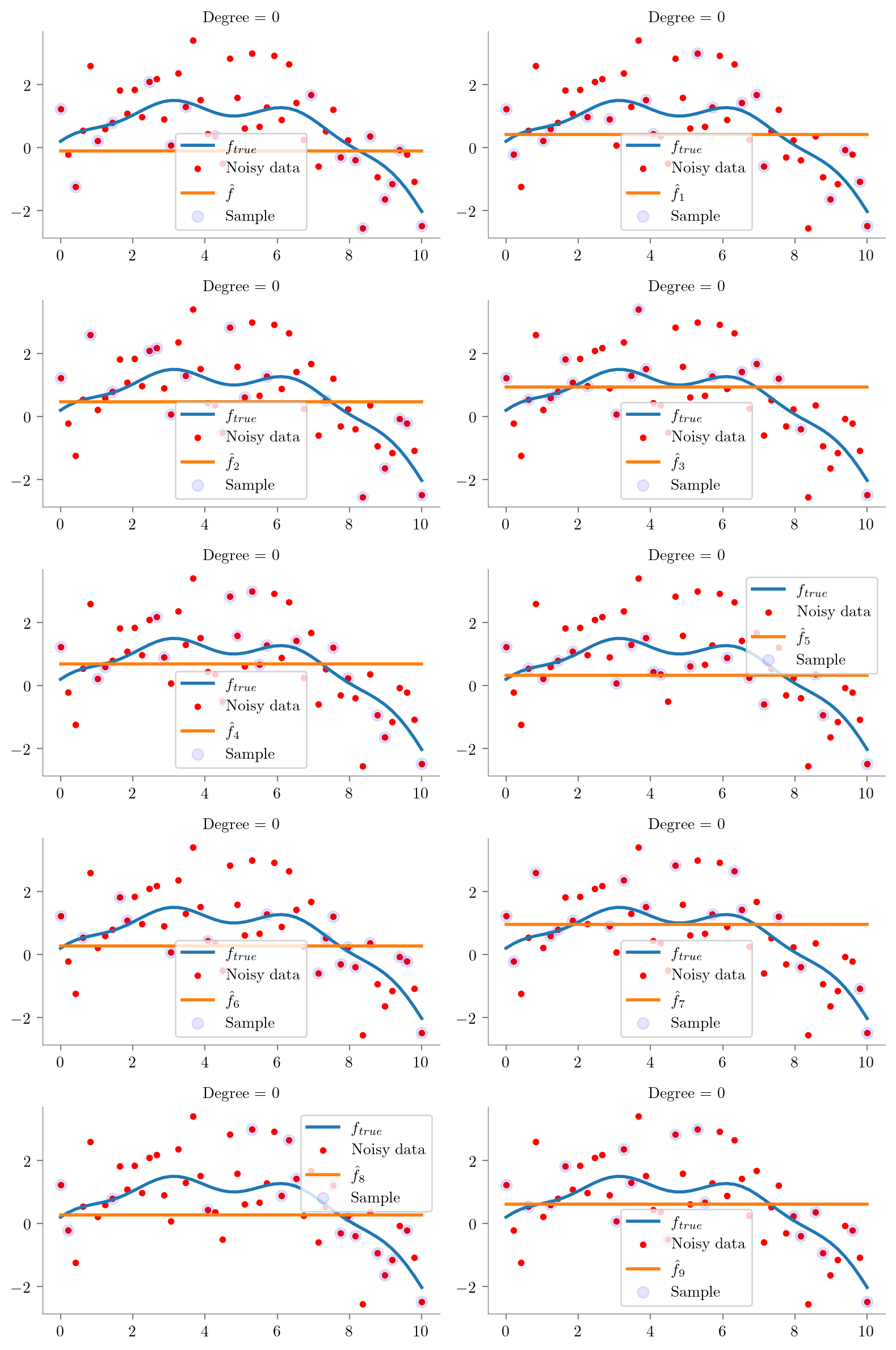

def plot_predictions(reg):
    x_test = np.linspace(0, 10, 50)
    y_pred = np.zeros((10, 50))
    for i in range(10):
        y_pred[i] = reg[i].predict(x_test.reshape(-1, 1))
    plt.plot(x_test, y_pred.mean(axis=0), label = r'$\hat{f}$', lw=2)
    plt.plot(x_test, f_x, label = r'$f_{true}$', lw=2)
    plt.plot(x_test, y_pred.T, lw=1, c='k', alpha=0.5)  
    format_axes(plt.gca())
    plt.legend()

plot_predictions(regs[1])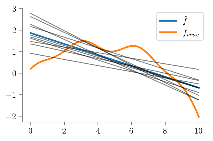

def plot_bias(reg):
    x_test = np.linspace(0, 10, 50)
    y_pred = np.zeros((10, 50))
    for i in range(10):
        y_pred[i] = reg[i].predict(x_test.reshape(-1, 1))
    y_pred_mean = np.mean(y_pred, axis=0)
    y_pred_var = np.var(y_pred, axis=0)

    plt.plot(x_overall, f_x, label = r'$f_{true}$', lw=2)
    #plt.scatter(x_overall, y_overall, s=10, c='r', label = 'Noisy data')
    plt.plot(x_test, y_pred_mean, label = r'$\bar{f}$', lw=2)
    plt.fill_between(x_test, y_pred_mean, f_x, alpha=0.2, color='green', label = 'Bias')
    plt.legend()

plot_bias(regs[7])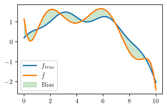

def plot_variance(reg):
    x_test = np.linspace(0, 10, 50)
    y_pred = np.zeros((10, 50))
    for i in range(10):
        y_pred[i] = reg[i].predict(x_test.reshape(-1, 1))
    y_pred_mean = np.mean(y_pred, axis=0)
    y_pred_var = np.var(y_pred, axis=0)

    plt.plot(x_overall, f_x, label = r'$f_{true}$', lw=2)
    #plt.scatter(x_overall, y_overall, s=10, c='r', label = 'Noisy data')
    plt.plot(x_test, y_pred_mean, label = r'$\bar{f}$', lw=2)
    plt.fill_between(x_test, y_pred_mean - y_pred_var, y_pred_mean + y_pred_var, alpha=0.2, color='red', label = 'Variance')
    plt.legend()

plot_variance(regs[8])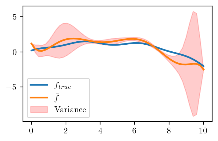

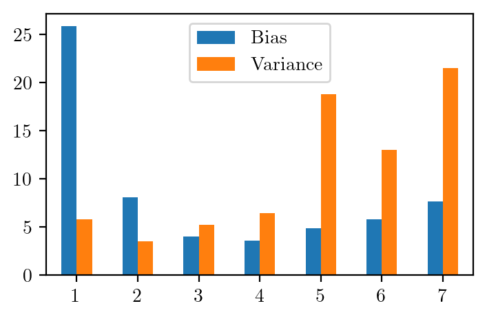
# Plot bias^2 and variance for different depths as bar plot

def plot_bias_variance(reg):
    x_test = np.linspace(0, 10, 50)
    y_pred = np.zeros((10, 50))
    for i in range(10):
        y_pred[i] = reg[i].predict(x_test.reshape(-1, 1))
    y_pred_mean = np.mean(y_pred, axis=0)
    y_pred_var = np.var(y_pred, axis=0)

    bias = (y_pred_mean - f_x)**2
    var = y_pred_var
    return bias.sum(), var.sum()

bs = {}
vs = {}
for i in range(1, 8):
    bs[i], vs[i] = plot_bias_variance(regs[i])

df = pd.DataFrame({'Bias': bs, 'Variance': vs})

df.plot.bar(rot=0)

Other Formats