Curse of Dimensionality

Author

Nipun Batra

Published

April 16, 2023

Open In Colab

import numpy as np
import matplotlib.pyplot as plt
import pandas as pd

%matplotlib inline
%config InlineBackend.figure_format = 'retina'

# 
n = 10
np.random.seed(42)
# Get `n` points in 1d space uniformly distributed from 0 to 1
x = np.random.uniform(0, 1, n)
plt.scatter(x, np.zeros(n), c='r', s=100)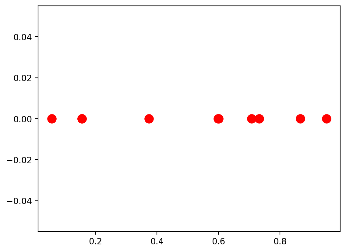

# Pick a random test point

x_test = np.random.uniform(0, 1, 1)


# Mark the nearest point and farthest point
x_nearest = x[np.argmin(np.abs(x - x_test))]
x_farthest = x[np.argmax(np.abs(x - x_test))]

plt.scatter(x, np.zeros(n), c='r', s=100)
plt.scatter(x_test, 0, c='b', s=100, marker='*', label='test')
plt.scatter(x_nearest, 0, c='g', s=100, label='nearest')
plt.scatter(x_farthest, 0, c='y', s=100, label='farthest')
plt.legend()

ratio = np.abs(x_test - x_nearest) / np.abs(x_test - x_farthest)
print('Ratio of distances: {}'.format(ratio))

Ratio of distances: [0.04356313]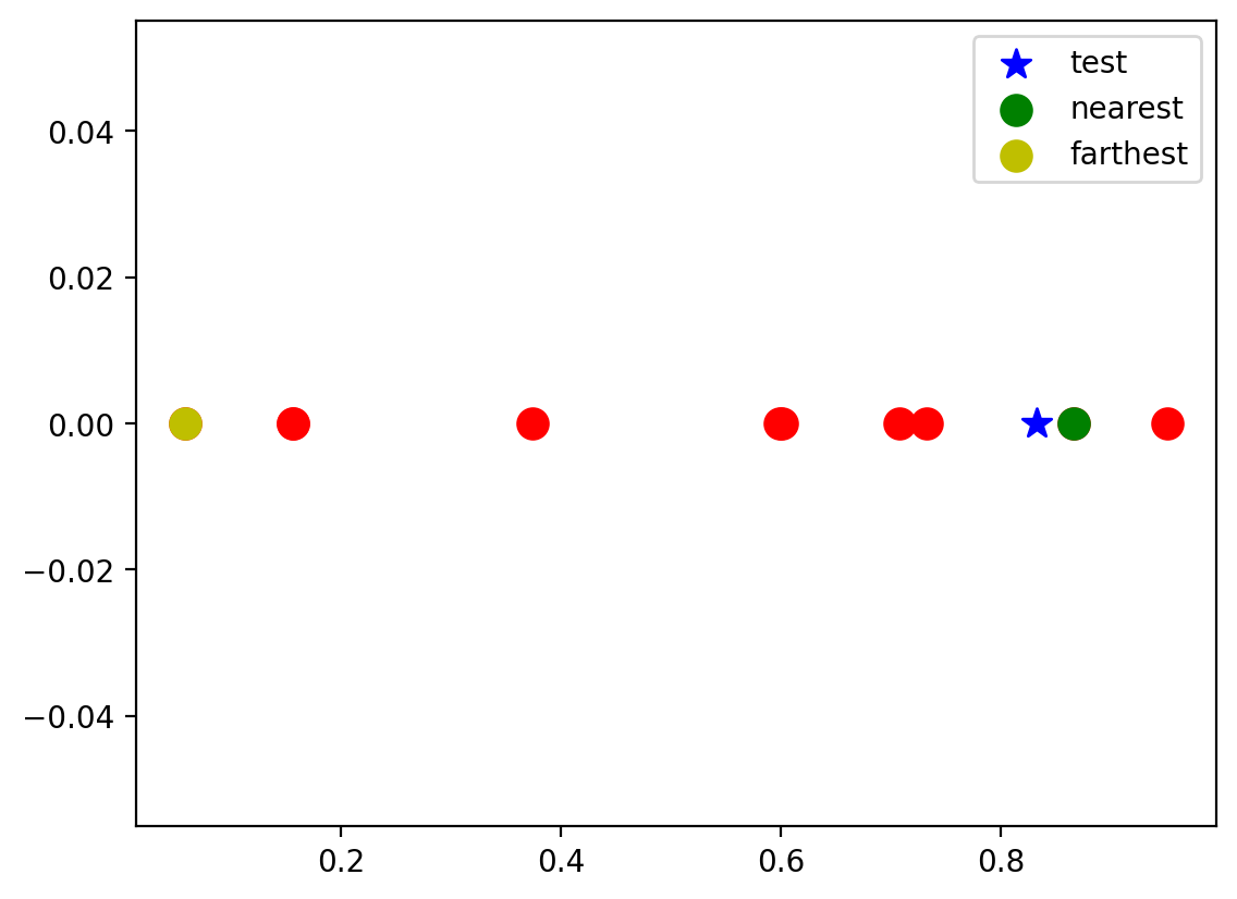

# Do the above experiment for 1000 times

n = 10
np.random.seed(42)

n_exp = 1000
ratios = np.zeros(n_exp)
for i in range(n_exp):
    x = np.random.uniform(0, 1, n)
    x_test = np.random.uniform(0, 1, 1)
    x_nearest = x[np.argmin(np.abs(x - x_test))]
    x_farthest = x[np.argmax(np.abs(x - x_test))]
    ratios[i] = np.abs(x_test - x_nearest) / np.abs(x_test - x_farthest)

import seaborn as sns
sns.displot(ratios, kde=False, bins=20)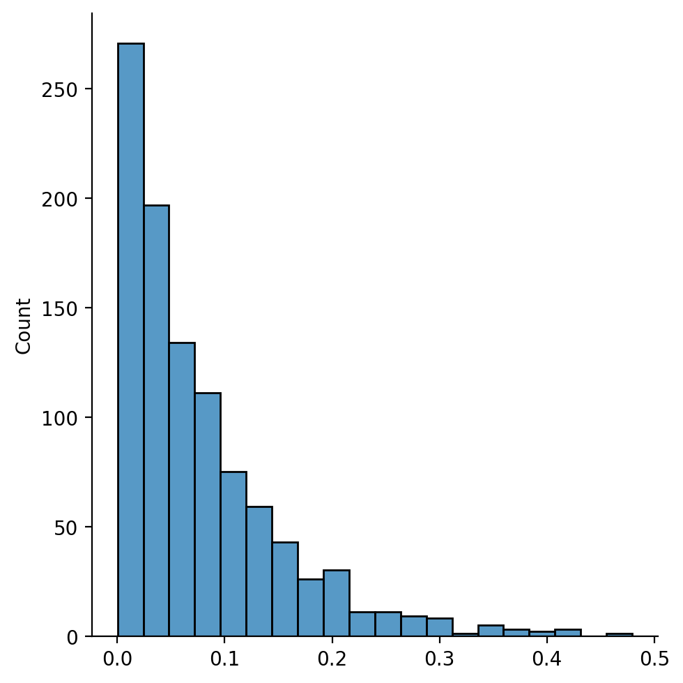

# Repeat the experiment in 2d

n = 10
np.random.seed(42)
x = np.random.uniform(0, 1, (n, 2))
plt.scatter(x[:, 0], x[:, 1], c='r', s=100)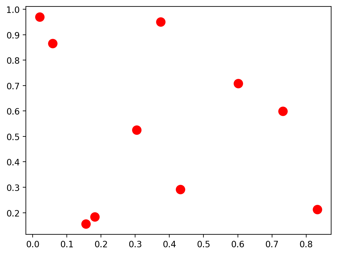

# Pick a random test point

x_test = np.random.uniform(0, 1, 2)

# Mark the nearest point and farthest point
x_nearest = x[np.argmin(np.linalg.norm(x - x_test, axis=1))]
x_farthest = x[np.argmax(np.linalg.norm(x - x_test, axis=1))]

plt.scatter(x[:, 0], x[:, 1], c='r', s=100)
plt.scatter(x_test[0], x_test[1], c='b', s=100, marker='*', label='test')
plt.scatter(x_nearest[0], x_nearest[1], c='g', s=100, label='nearest')
plt.scatter(x_farthest[0], x_farthest[1], c='y', s=100, label='farthest')
plt.legend()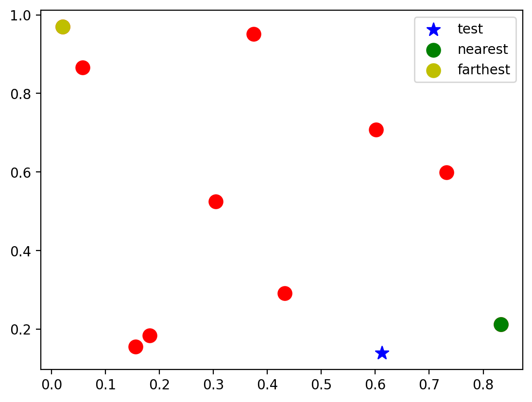

# Find the ratio of distances between the nearest and farthest points in 1000 experiments

n = 10
np.random.seed(42)

ratios_2d = np.zeros(n_exp)
for i in range(n_exp):
    x = np.random.uniform(0, 1, (n, 2))
    x_test = np.random.uniform(0, 1, 2)
    x_nearest = x[np.argmin(np.linalg.norm(x - x_test, axis=1))]
    x_farthest = x[np.argmax(np.linalg.norm(x - x_test, axis=1))]
    ratios_2d[i] = np.linalg.norm(x_test - x_nearest) / np.linalg.norm(x_test - x_farthest)

sns.displot(ratios_2d, kde=False, bins=20)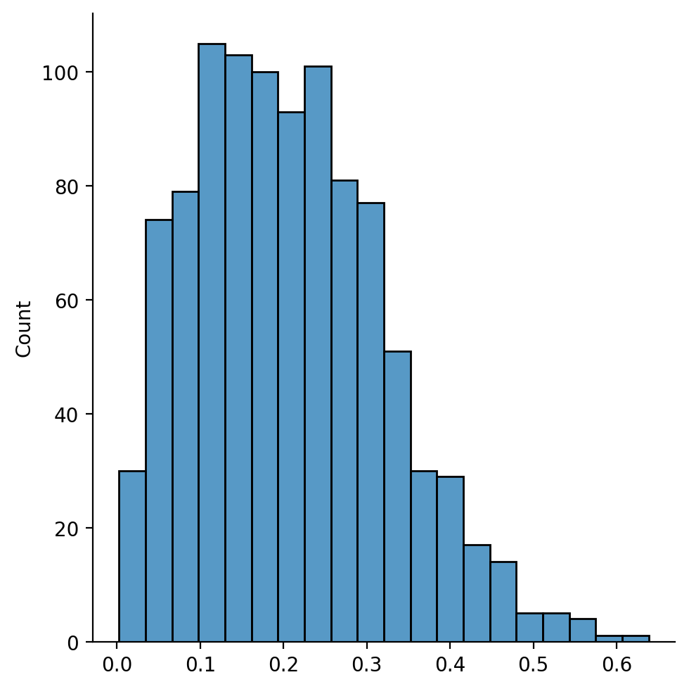

# Now, let's do the same experiment in dimensions varying from 1 to 20

n = 10
np.random.seed(42)
n_dim = 101
ratios_nd = np.zeros((n_exp, n_dim))
for i in range(n_exp):
    for d in range(1, n_dim + 1):
        x = np.random.uniform(0, 1, (n, d))
        x_test = np.random.uniform(0, 1, d)
        x_nearest = x[np.argmin(np.linalg.norm(x - x_test, axis=1))]
        x_farthest = x[np.argmax(np.linalg.norm(x - x_test, axis=1))]
        ratios_nd[i, d - 1] = np.linalg.norm(x_test - x_nearest) / np.linalg.norm(x_test - x_farthest)

# Plot the ratio of distances between the nearest and farthest points in 1000 experiments for each dimension

from matplotlib import markers


plt.figure(figsize=(10, 6))
plt.plot(np.arange(1, n_dim + 1), np.mean(ratios_nd, axis=0), 'o-', markersize=3)
plt.xlabel('Dimension')
plt.ylabel('Ratio of distances')
plt.title('Ratio of distances between the nearest and farthest points in 1000 experiments for each dimension')
plt.ylim(0, 1.)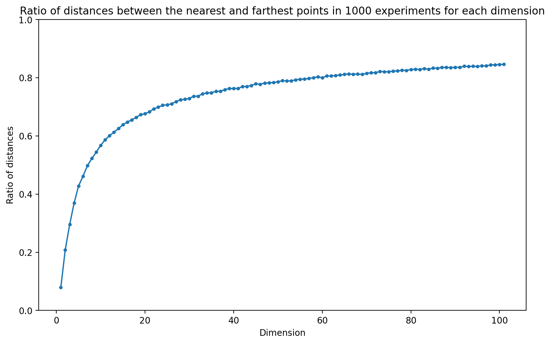

# Let us now see what happens if we have more points in higher dimensions
# 1d space: 10 points

n = 10
np.random.seed(42)
n_dim = 4
ratios_nd_more_points = np.zeros((n_exp, n_dim))
num_points = [10, 50, 200, 2000]
for i in range(n_exp):
    for d in range(1, n_dim + 1):
        x = np.random.uniform(0, 1, (num_points[d-1], d))
        x_test = np.random.uniform(0, 1, d)
        x_nearest = x[np.argmin(np.linalg.norm(x - x_test, axis=1))]
        x_farthest = x[np.argmax(np.linalg.norm(x - x_test, axis=1))]
        ratios_nd_more_points[i, d - 1] = np.linalg.norm(x_test - x_nearest) / np.linalg.norm(x_test - x_farthest)

import pandas as pd
cols = [(1, 10), (2, 50), (3, 200), (4, 2000)]
df = pd.DataFrame(ratios_nd_more_points, columns=cols)
df

	(1, 10)	(2, 50)	(3, 200)	(4, 2000)
0	0.040316	0.040880	0.081673	0.055671
1	0.056051	0.094828	0.139413	0.063989
2	0.098272	0.076760	0.163102	0.078649
3	0.213181	0.165776	0.055523	0.033316
4	0.011092	0.105754	0.070214	0.081415
...	...	...	...	...
995	0.005806	0.108972	0.075787	0.104469
996	0.178349	0.056938	0.067411	0.047147
997	0.006966	0.070710	0.061830	0.095790
998	0.047800	0.082439	0.095661	0.049558
999	0.080716	0.042173	0.033175	0.082464

1000 rows × 4 columns

df.mean().plot(kind='bar', rot=0)
plt.ylabel('Ratio of distances')
plt.xlabel('Dimension, number of points')
_= plt.title('Ratio of distances between the nearest and farthest points \nin 1000 experiments for each dimension and number of points')
plt.ylim(0, 1.)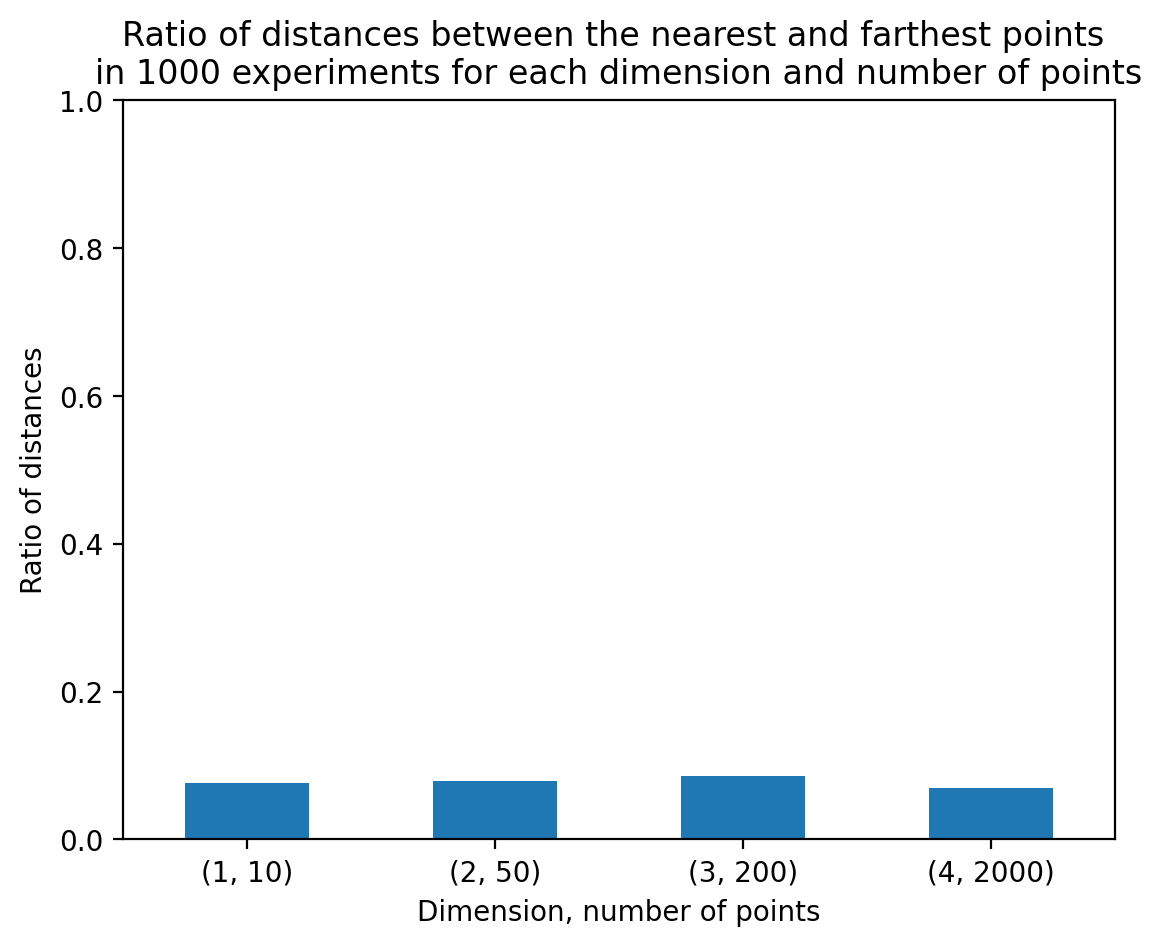

# Now showing how linear regression is affected by curse of dimensionality

n_points = 20

x = np.random.uniform(0, 1, (n_points, 1))
# sort the x values
x = np.sort(x, axis=0)
y = 4 * x + 3 + np.random.normal(0, 0.5, (n_points, 1))

plt.scatter(x, y)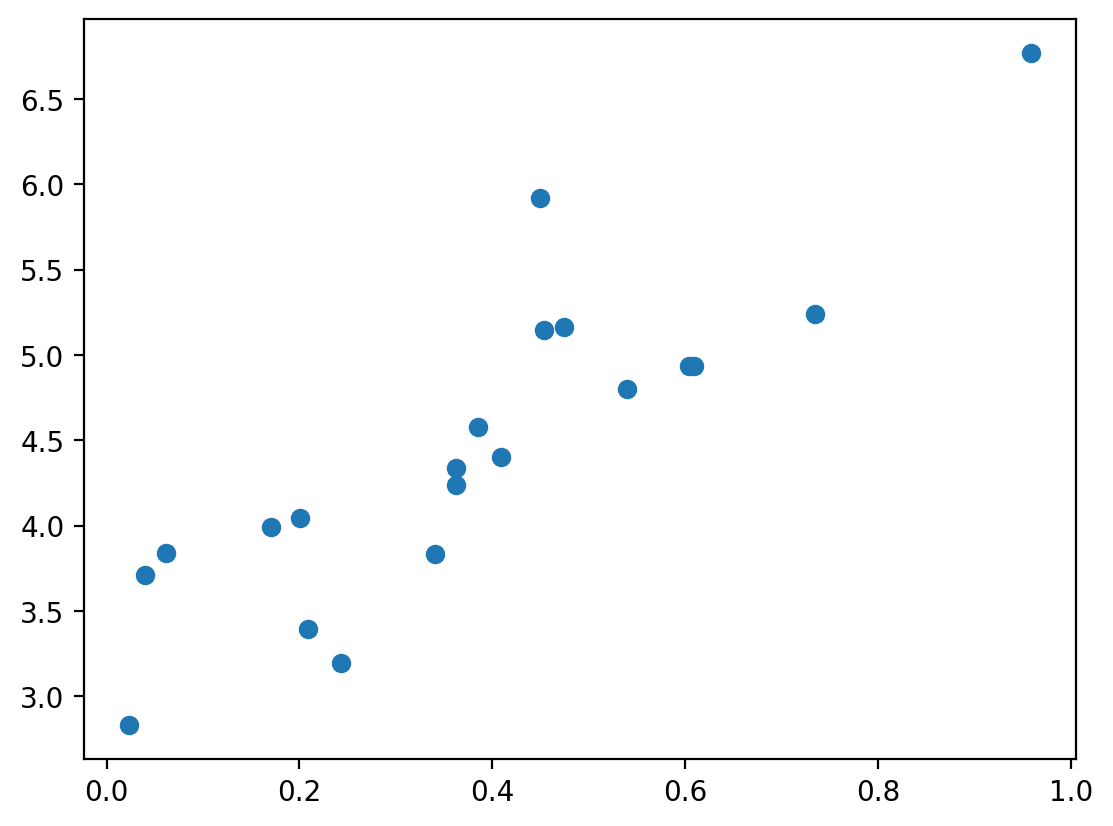

# Let us fit a linear regression model of degree d
from sklearn.linear_model import LinearRegression
from sklearn.preprocessing import PolynomialFeatures

def fit_linear_regression(x, y, d):
    poly = PolynomialFeatures(degree=d)
    x = poly.fit_transform(x)
    model = LinearRegression()
    model.fit(x, y)
    return model

def plot_linear_regression(x, y, d):
    model = fit_linear_regression(x, y, d)
    y_pred = model.predict(PolynomialFeatures(degree=d).fit_transform(x))
    plt.scatter(x, y)
    plt.plot(x, y_pred, c='r')
    plt.show()

plot_linear_regression(x, y, 1)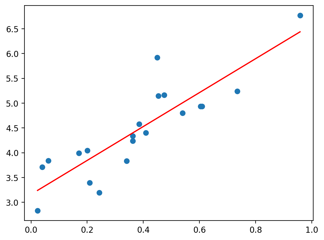

plot_linear_regression(x, y, 5)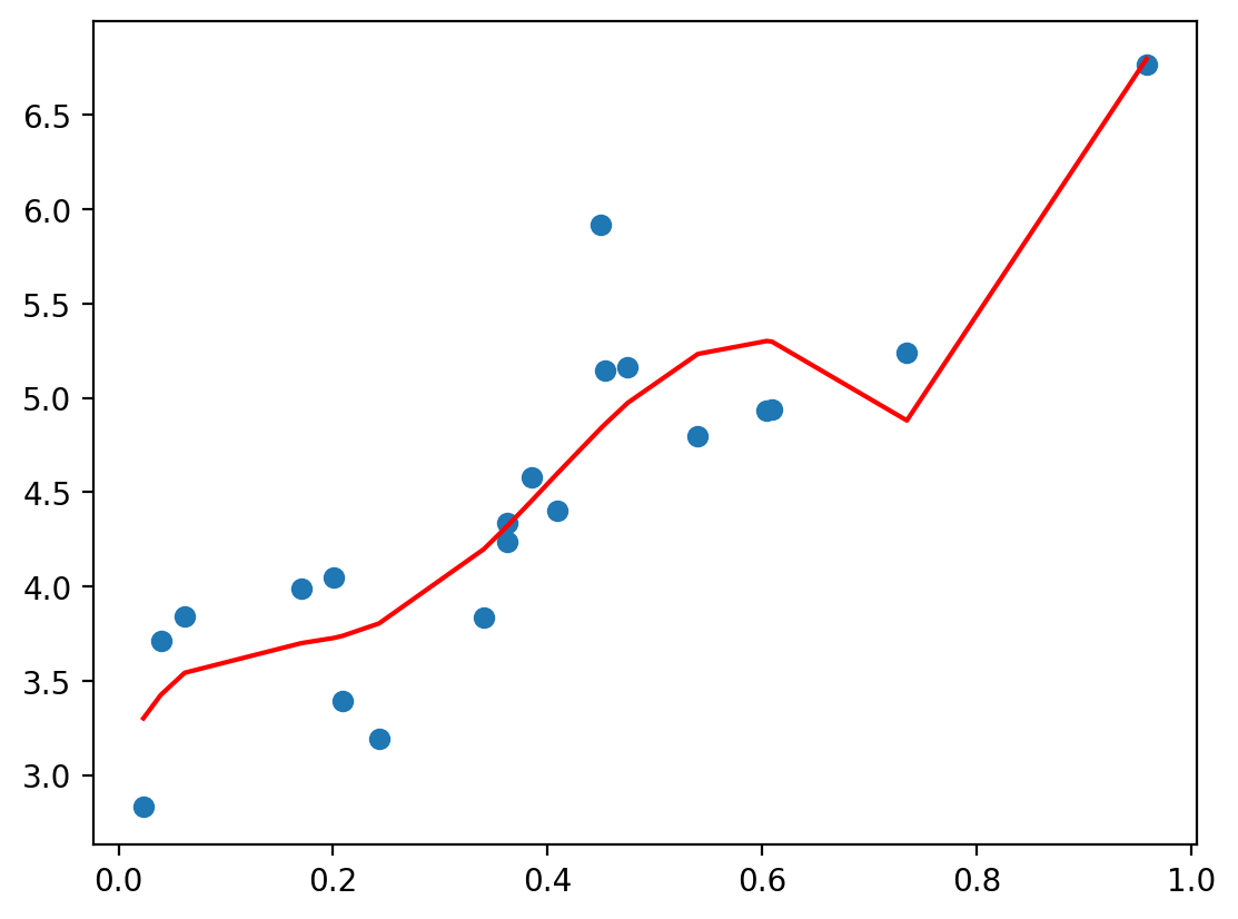

plot_linear_regression(x, y, 10)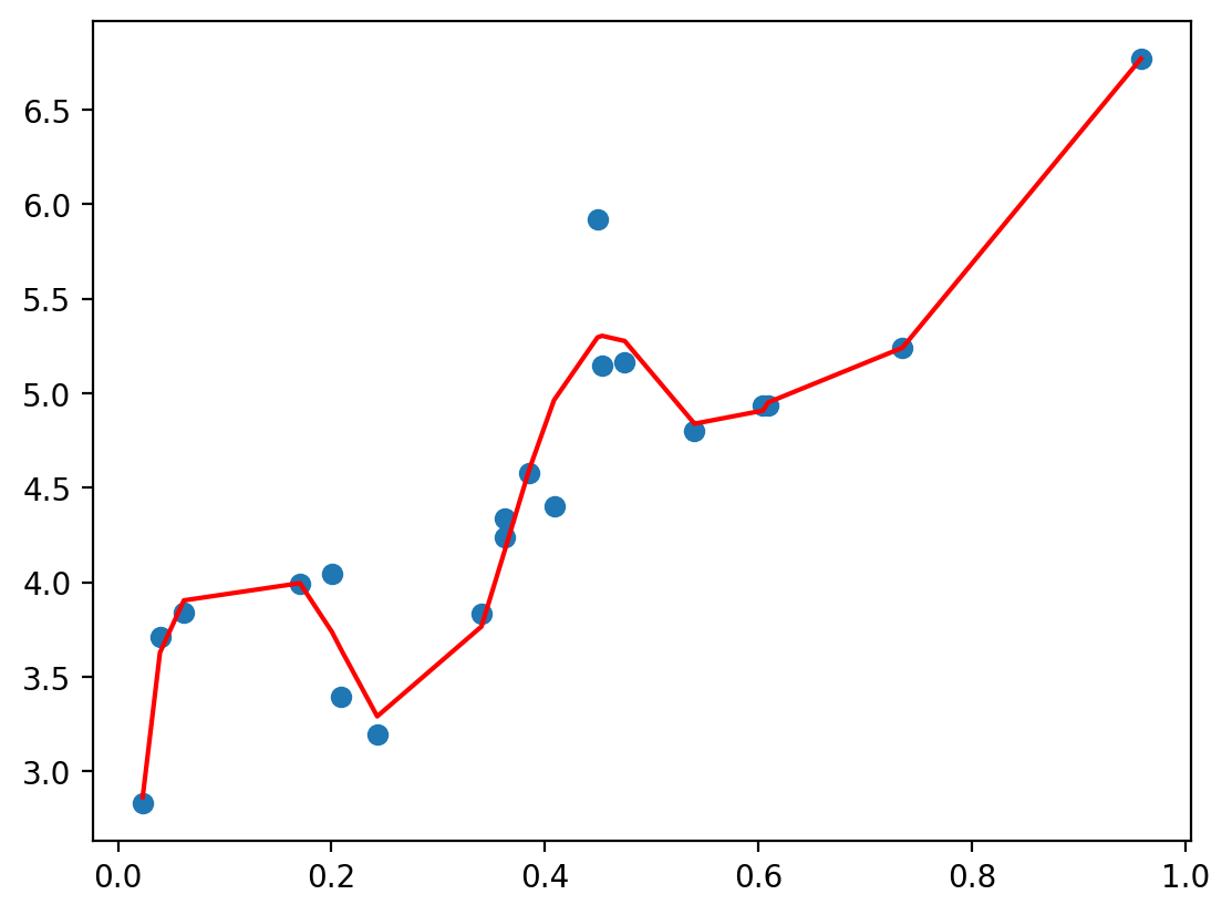

plot_linear_regression(x, y, 15)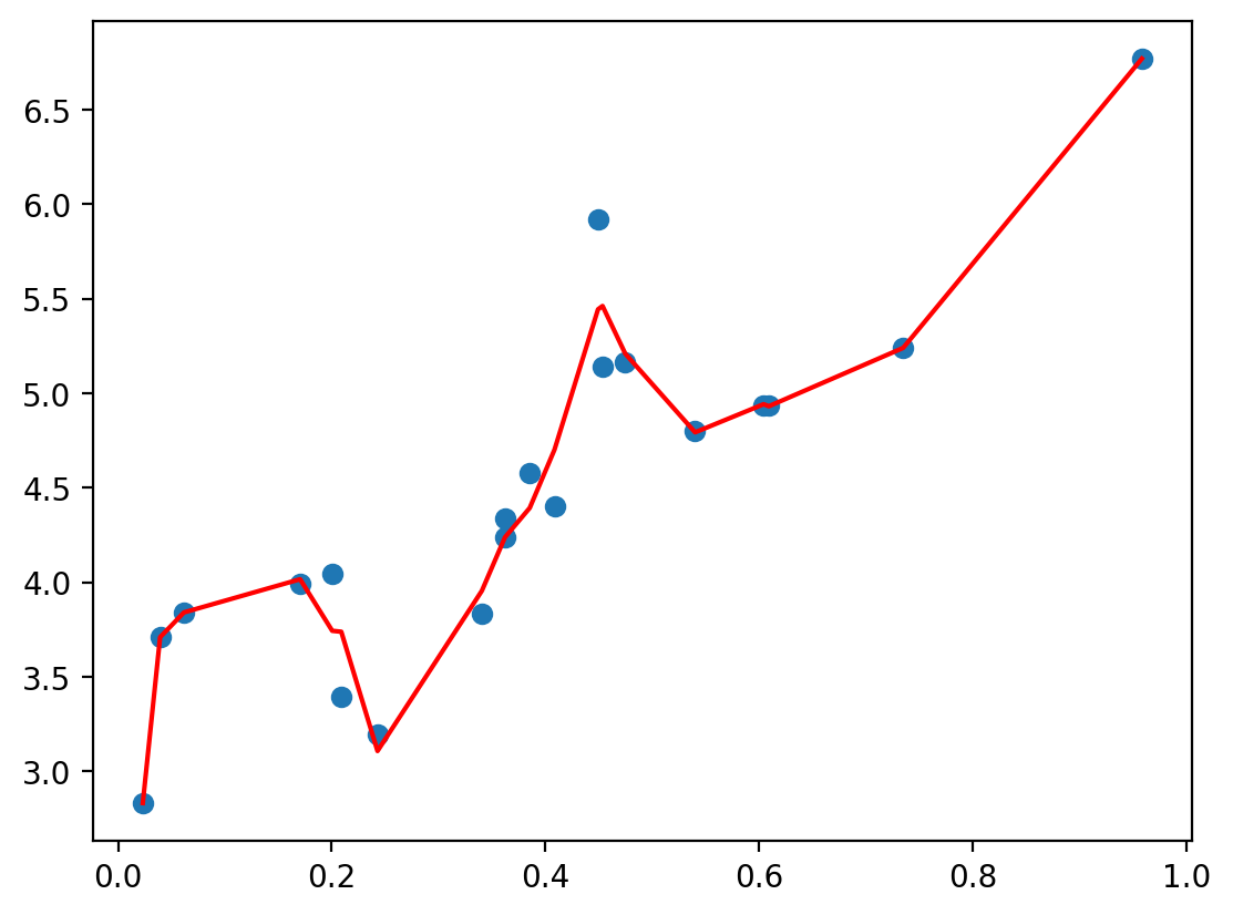

# Now, we see that if we increase the number of points, the model will fit better

n_points = 1000

x = np.random.uniform(0, 1, (n_points, 1))
# sort the x values
x = np.sort(x, axis=0)
y = 4 * x + 3 + np.random.normal(0, 0.5, (n_points, 1))

plot_linear_regression(x, y, 1)

plot_linear_regression(x, y, 5)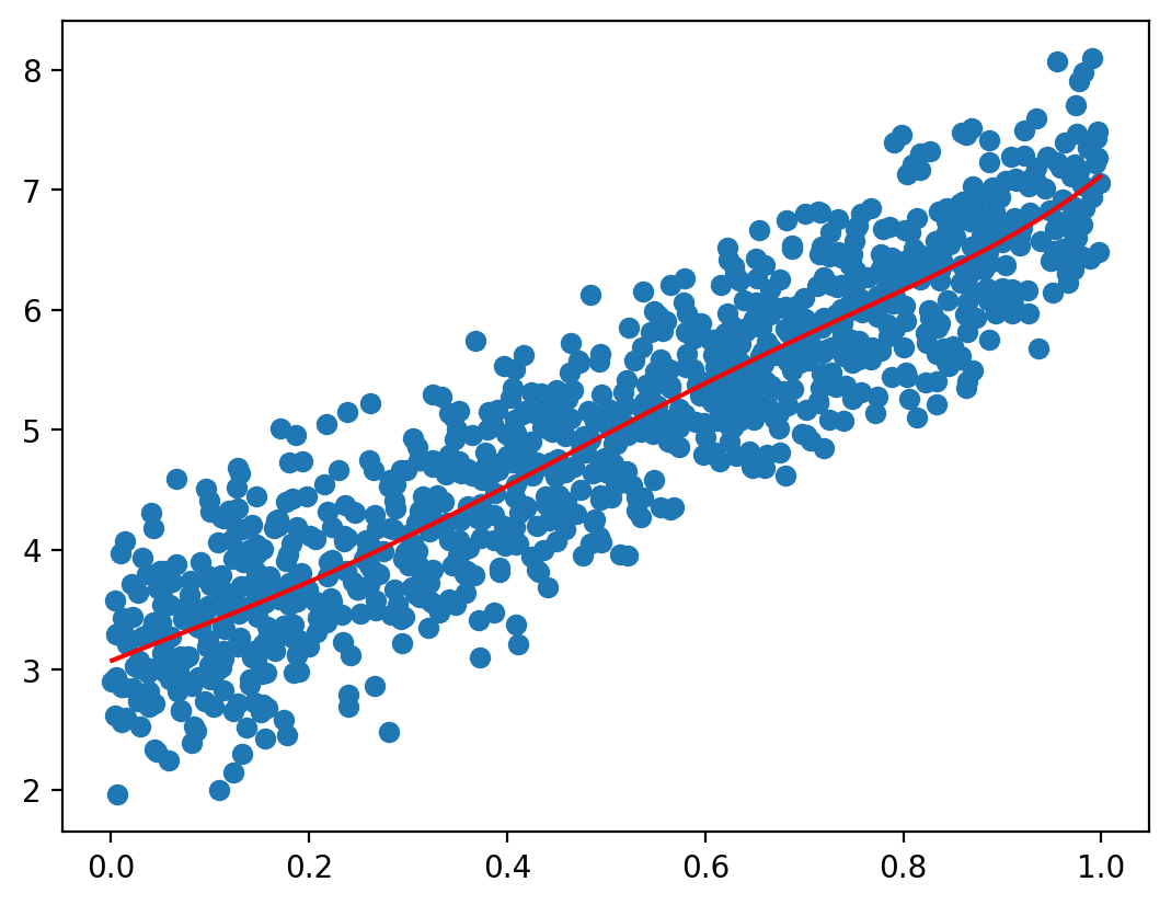

plot_linear_regression(x, y, 25)

Other Formats