DECISION TREE PRUNING

import sklearn
sklearn.__version__

'1.6.1'

import matplotlib.pyplot as plt
from sklearn.model_selection import train_test_split
from sklearn.datasets import load_breast_cancer
from sklearn.tree import plot_tree
from sklearn.tree import DecisionTreeRegressor
from sklearn.tree import DecisionTreeClassifier

data = load_breast_cancer()
print(data.DESCR)

.. _breast_cancer_dataset:

Breast cancer wisconsin (diagnostic) dataset
--------------------------------------------

**Data Set Characteristics:**

:Number of Instances: 569

:Number of Attributes: 30 numeric, predictive attributes and the class

:Attribute Information:
    - radius (mean of distances from center to points on the perimeter)
    - texture (standard deviation of gray-scale values)
    - perimeter
    - area
    - smoothness (local variation in radius lengths)
    - compactness (perimeter^2 / area - 1.0)
    - concavity (severity of concave portions of the contour)
    - concave points (number of concave portions of the contour)
    - symmetry
    - fractal dimension ("coastline approximation" - 1)

    The mean, standard error, and "worst" or largest (mean of the three
    worst/largest values) of these features were computed for each image,
    resulting in 30 features.  For instance, field 0 is Mean Radius, field
    10 is Radius SE, field 20 is Worst Radius.

    - class:
            - WDBC-Malignant
            - WDBC-Benign

:Summary Statistics:

===================================== ====== ======
                                        Min    Max
===================================== ====== ======
radius (mean):                        6.981  28.11
texture (mean):                       9.71   39.28
perimeter (mean):                     43.79  188.5
area (mean):                          143.5  2501.0
smoothness (mean):                    0.053  0.163
compactness (mean):                   0.019  0.345
concavity (mean):                     0.0    0.427
concave points (mean):                0.0    0.201
symmetry (mean):                      0.106  0.304
fractal dimension (mean):             0.05   0.097
radius (standard error):              0.112  2.873
texture (standard error):             0.36   4.885
perimeter (standard error):           0.757  21.98
area (standard error):                6.802  542.2
smoothness (standard error):          0.002  0.031
compactness (standard error):         0.002  0.135
concavity (standard error):           0.0    0.396
concave points (standard error):      0.0    0.053
symmetry (standard error):            0.008  0.079
fractal dimension (standard error):   0.001  0.03
radius (worst):                       7.93   36.04
texture (worst):                      12.02  49.54
perimeter (worst):                    50.41  251.2
area (worst):                         185.2  4254.0
smoothness (worst):                   0.071  0.223
compactness (worst):                  0.027  1.058
concavity (worst):                    0.0    1.252
concave points (worst):               0.0    0.291
symmetry (worst):                     0.156  0.664
fractal dimension (worst):            0.055  0.208
===================================== ====== ======

:Missing Attribute Values: None

:Class Distribution: 212 - Malignant, 357 - Benign

:Creator:  Dr. William H. Wolberg, W. Nick Street, Olvi L. Mangasarian

:Donor: Nick Street

:Date: November, 1995

This is a copy of UCI ML Breast Cancer Wisconsin (Diagnostic) datasets.
https://goo.gl/U2Uwz2

Features are computed from a digitized image of a fine needle
aspirate (FNA) of a breast mass.  They describe
characteristics of the cell nuclei present in the image.

Separating plane described above was obtained using
Multisurface Method-Tree (MSM-T) [K. P. Bennett, "Decision Tree
Construction Via Linear Programming." Proceedings of the 4th
Midwest Artificial Intelligence and Cognitive Science Society,
pp. 97-101, 1992], a classification method which uses linear
programming to construct a decision tree.  Relevant features
were selected using an exhaustive search in the space of 1-4
features and 1-3 separating planes.

The actual linear program used to obtain the separating plane
in the 3-dimensional space is that described in:
[K. P. Bennett and O. L. Mangasarian: "Robust Linear
Programming Discrimination of Two Linearly Inseparable Sets",
Optimization Methods and Software 1, 1992, 23-34].

This database is also available through the UW CS ftp server:

ftp ftp.cs.wisc.edu
cd math-prog/cpo-dataset/machine-learn/WDBC/

.. dropdown:: References

  - W.N. Street, W.H. Wolberg and O.L. Mangasarian. Nuclear feature extraction
    for breast tumor diagnosis. IS&T/SPIE 1993 International Symposium on
    Electronic Imaging: Science and Technology, volume 1905, pages 861-870,
    San Jose, CA, 1993.
  - O.L. Mangasarian, W.N. Street and W.H. Wolberg. Breast cancer diagnosis and
    prognosis via linear programming. Operations Research, 43(4), pages 570-577,
    July-August 1995.
  - W.H. Wolberg, W.N. Street, and O.L. Mangasarian. Machine learning techniques
    to diagnose breast cancer from fine-needle aspirates. Cancer Letters 77 (1994)
    163-171.

X, y = load_breast_cancer(return_X_y=True)
X_train, X_test, y_train, y_test = train_test_split(X, y, random_state=0)

X_train.shape

(426, 30)

unpruned_tree = DecisionTreeClassifier(random_state=0)
unpruned_tree.fit(X_train,y_train)

DecisionTreeClassifier(random_state=0)

In a Jupyter environment, please rerun this cell to show the HTML representation or trust the notebook.
On GitHub, the HTML representation is unable to render, please try loading this page with nbviewer.org.

pred=unpruned_tree.predict(X_test)
from sklearn.metrics import accuracy_score
print("Test Accuracy ->",accuracy_score(y_test, pred))

Test Accuracy -> 0.8811188811188811

print("Train Accuracy ->",unpruned_tree.score(X_train, y_train))

Train Accuracy -> 1.0

from sklearn import tree
plt.figure(figsize=(15,10))
tree.plot_tree(unpruned_tree,filled=True)
plt.title("Unpruned Decision Tree")

Text(0.5, 1.0, 'Unpruned Decision Tree')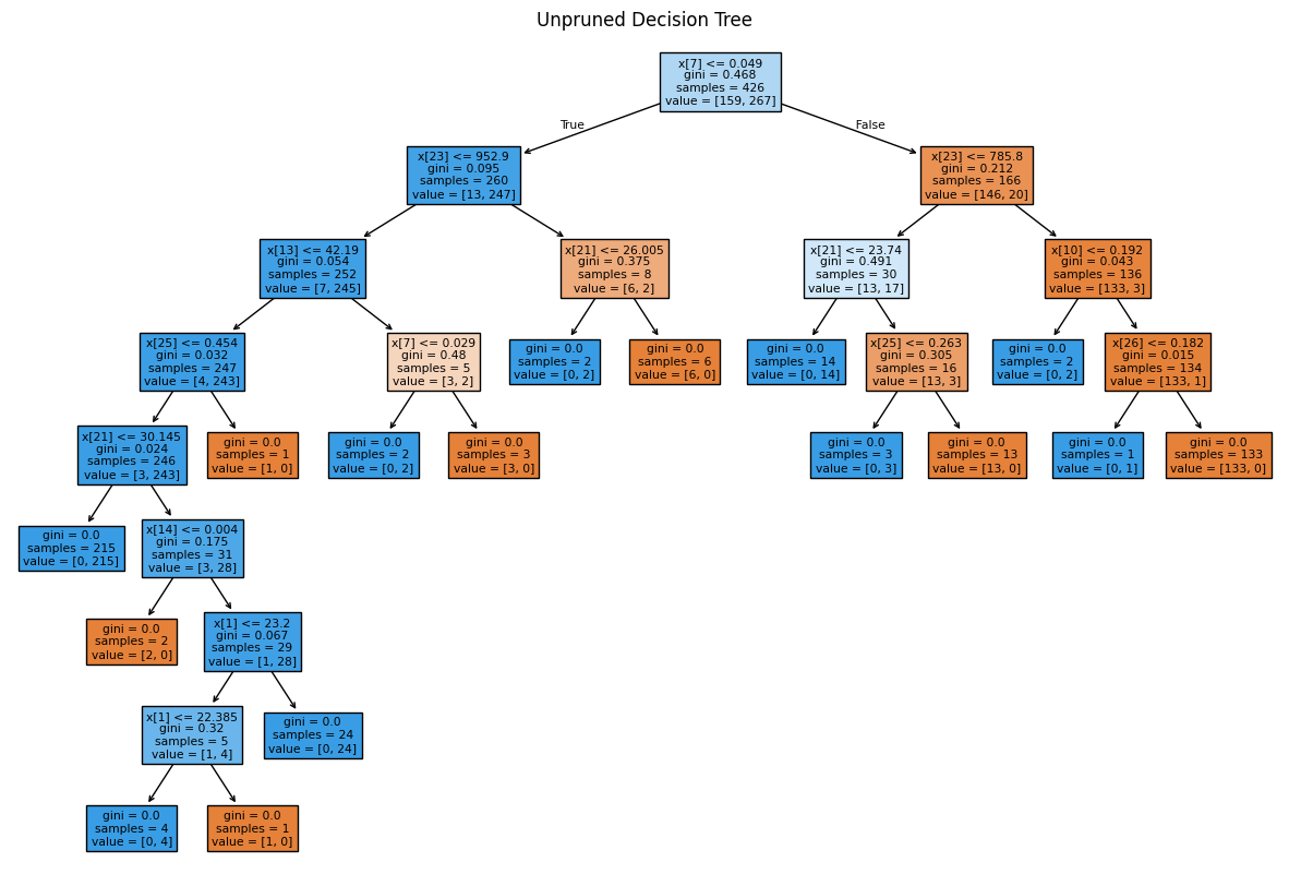

Pre Pruning

The class:DecisionTreeClassifier takes parameters such as min_samples_leaf and max_depth to prevent a tree from overfitting.

print(unpruned_tree.get_params())

{'ccp_alpha': 0.0, 'class_weight': None, 'criterion': 'gini', 'max_depth': None, 'max_features': None, 'max_leaf_nodes': None, 'min_impurity_decrease': 0.0, 'min_samples_leaf': 1, 'min_samples_split': 2, 'min_weight_fraction_leaf': 0.0, 'monotonic_cst': None, 'random_state': 0, 'splitter': 'best'}


pre_pruned_tree = DecisionTreeClassifier(max_leaf_nodes=4,random_state=0)
pre_pruned_tree.fit(X_train,y_train)

DecisionTreeClassifier(max_leaf_nodes=4, random_state=0)

print("Train Accuracy ->",pre_pruned_tree.score(X_train, y_train))

Train Accuracy -> 0.9553990610328639

pred=pre_pruned_tree.predict(X_test)
print("Test accuracy ->",accuracy_score(y_test, pred))

Test accuracy -> 0.916083916083916

plt.figure(figsize=(15,8))
tree.plot_tree(pre_pruned_tree,filled=True)
plt.title("Pre-pruned Decision Tree")

Text(0.5, 1.0, 'Pre-pruned Decision Tree')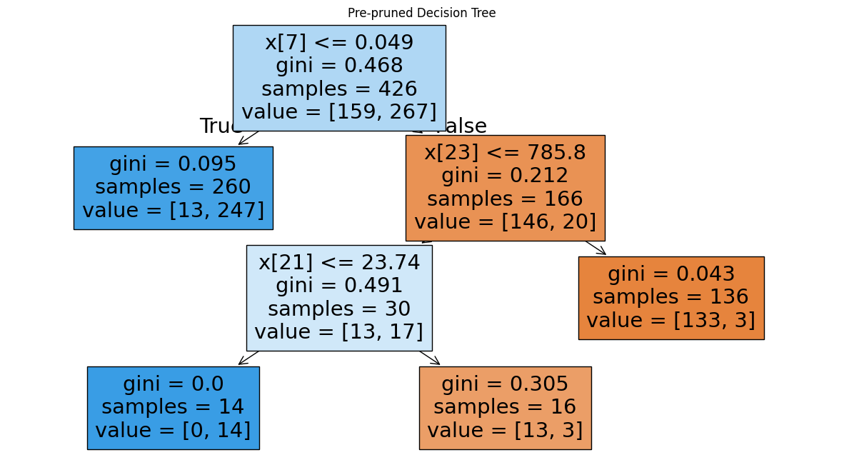

Post pruning

Cost complexity pruning is used to control the size of a tree. In :class:DecisionTreeClassifier, this pruning technique is parameterized by the cost complexity parameter, ccp_alpha. Greater values of ccp_alpha increase the number of nodes pruned. Here we show the effect of ccp_alpha on regularizing the trees and how to choose a ccp_alpha based on validation scores.

path = unpruned_tree.cost_complexity_pruning_path(X_train, y_train)
ccp_alphas, impurities = path.ccp_alphas, path.impurities

path

{'ccp_alphas': array([0.        , 0.00226647, 0.00464743, 0.0046598 , 0.0056338 ,
        0.00704225, 0.00784194, 0.00911402, 0.01144366, 0.018988  ,
        0.02314163, 0.03422475, 0.32729844]),
 'impurities': array([0.        , 0.00453294, 0.01847522, 0.02313502, 0.02876883,
        0.03581108, 0.04365302, 0.05276704, 0.0642107 , 0.0831987 ,
        0.10634033, 0.14056508, 0.46786352])}

ccp_alphas

array([0.        , 0.00226647, 0.00464743, 0.0046598 , 0.0056338 ,
       0.00704225, 0.00784194, 0.00911402, 0.01144366, 0.018988  ,
       0.02314163, 0.03422475, 0.32729844])

impurities

array([0.        , 0.00453294, 0.01847522, 0.02313502, 0.02876883,
       0.03581108, 0.04365302, 0.05276704, 0.0642107 , 0.0831987 ,
       0.10634033, 0.14056508, 0.46786352])

clfs = []
for ccp_alpha in ccp_alphas:
    clf = DecisionTreeClassifier(random_state=0, ccp_alpha=ccp_alpha)
    clf.fit(X_train, y_train)
    clfs.append(clf)
print("Number of nodes in the last tree is: {} with ccp_alpha: {}".format(
      clfs[-1].tree_.node_count, ccp_alphas[-1]))

Number of nodes in the last tree is: 1 with ccp_alpha: 0.3272984419327777

import io
import imageio
import matplotlib.pyplot as plt
from sklearn import tree

images = []
for i, clf in enumerate(clfs):
    buf = io.BytesIO()
    plt.figure(figsize=(10, 8))
    tree.plot_tree(clf, filled=True, fontsize=6)
    plt.title(f"Tree with ccp_alpha={ccp_alphas[i]:.4f}")
    plt.savefig(buf, format='png')
    plt.close()

    images.append(imageio.imread(buf))

imageio.mimsave('pruned_trees_in_memory.gif', images, duration=1000) # Increased duration to 10 seconds
from IPython.display import Image
Image(filename='pruned_trees_in_memory.gif',embed=True)

<IPython.core.display.Image object>

Total Impurity Vs Alpha

fig, ax = plt.subplots(figsize=(15, 8))
ax.plot(ccp_alphas[:-1], impurities[:-1], marker="o", drawstyle="steps-post")
ax.set_xlabel("effective alpha")
ax.set_ylabel("total impurity of leaves")
ax.set_title("Total Impurity vs effective alpha for training set")

Text(0.5, 1.0, 'Total Impurity vs effective alpha for training set')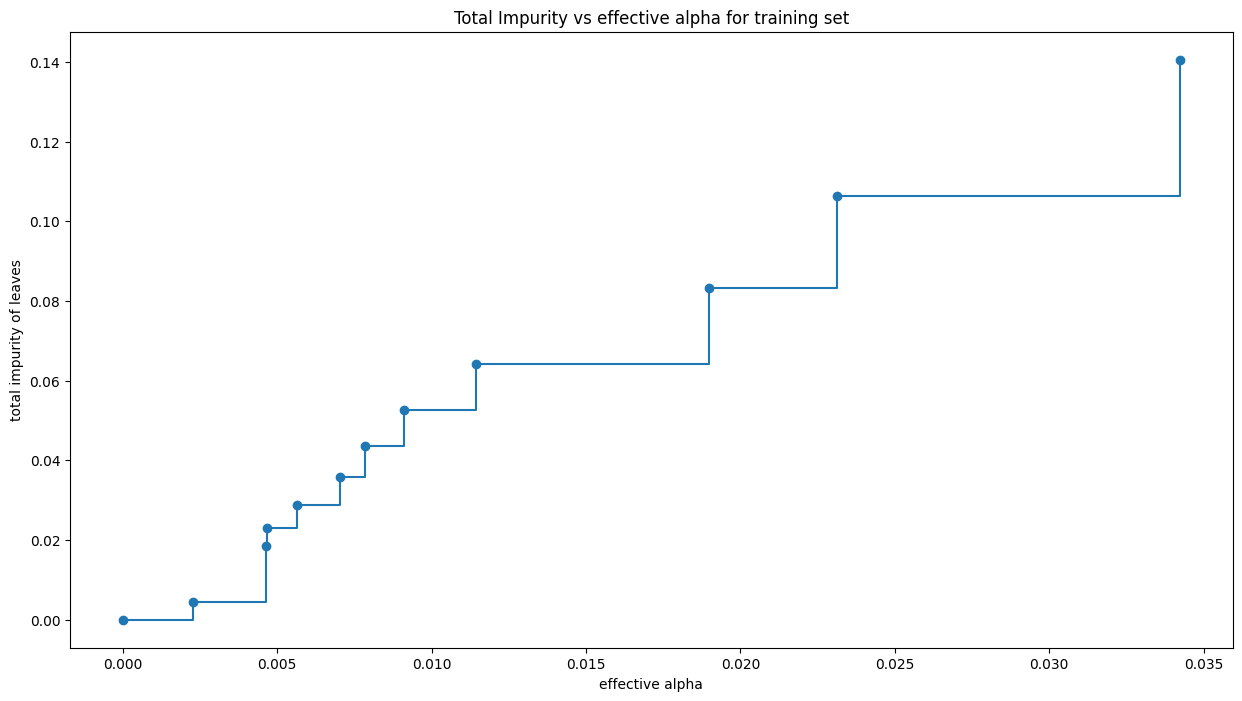

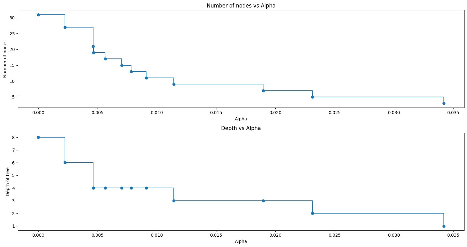
For this plot, we remove the last element in clfs and ccp_alphas, because it is the trivial tree with only one node. .

Number of nodes Vs Alpha

clfs = clfs[:-1]
ccp_alphas = ccp_alphas[:-1]

node_counts = [clf.tree_.node_count for clf in clfs]
depth = [clf.tree_.max_depth for clf in clfs]
fig, ax = plt.subplots(2, 1,figsize=(15, 8))
ax[0].plot(ccp_alphas, node_counts, marker="o", drawstyle="steps-post")
ax[0].set_xlabel("Alpha")
ax[0].set_ylabel("Number of nodes")
ax[0].set_title("Number of nodes vs Alpha")
ax[1].plot(ccp_alphas, depth, marker="o", drawstyle="steps-post")
ax[1].set_xlabel("Alpha")
ax[1].set_ylabel("Depth of tree")
ax[1].set_title("Depth vs Alpha")
fig.tight_layout()

Accuracy Vs Alpha

train_scores = [clf.score(X_train, y_train) for clf in clfs]
test_scores = [clf.score(X_test, y_test) for clf in clfs]

fig, ax = plt.subplots(figsize=(15, 8))
ax.set_xlabel("alpha")
ax.set_ylabel("accuracy")
ax.set_title("Accuracy vs alpha for training and testing sets")
ax.plot(ccp_alphas, train_scores, marker='o', label="Train",
        drawstyle="steps-post")
ax.plot(ccp_alphas, test_scores, marker='o', label="Test",
        drawstyle="steps-post")

optimal_alpha_index = test_scores.index(max(test_scores))
optimal_alpha = ccp_alphas[optimal_alpha_index]
highest_test_score = test_scores[optimal_alpha_index]


ax.plot(optimal_alpha, highest_test_score, 'o', color='red', markersize=15, fillstyle='none', label=f'Highest Test Accuracy (alpha={optimal_alpha:.4f})')

ax.hlines(highest_test_score, ax.get_xlim()[0], optimal_alpha, color='gray', linestyle='--', alpha=0.7)
ax.vlines(optimal_alpha, ax.get_ylim()[0], highest_test_score, color='gray', linestyle='--', alpha=0.7)


ax.legend()
plt.show()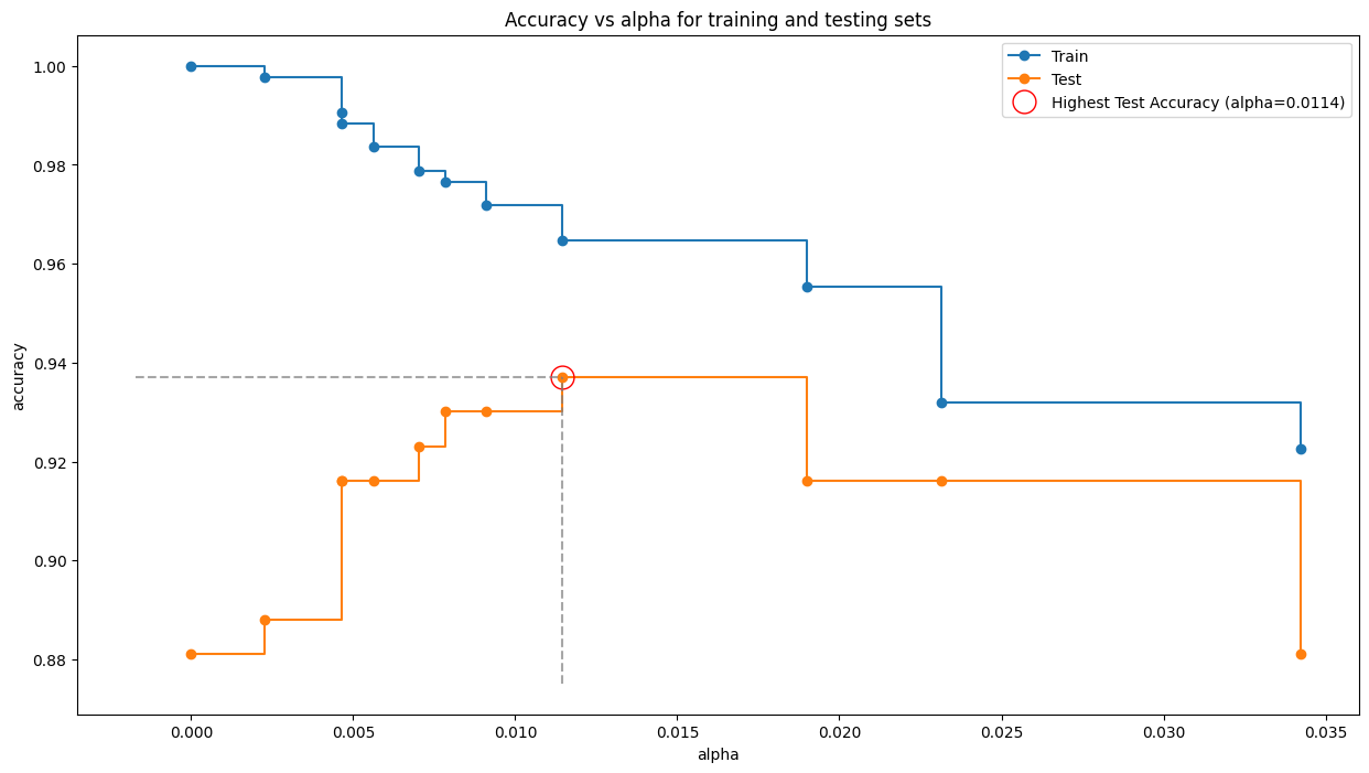

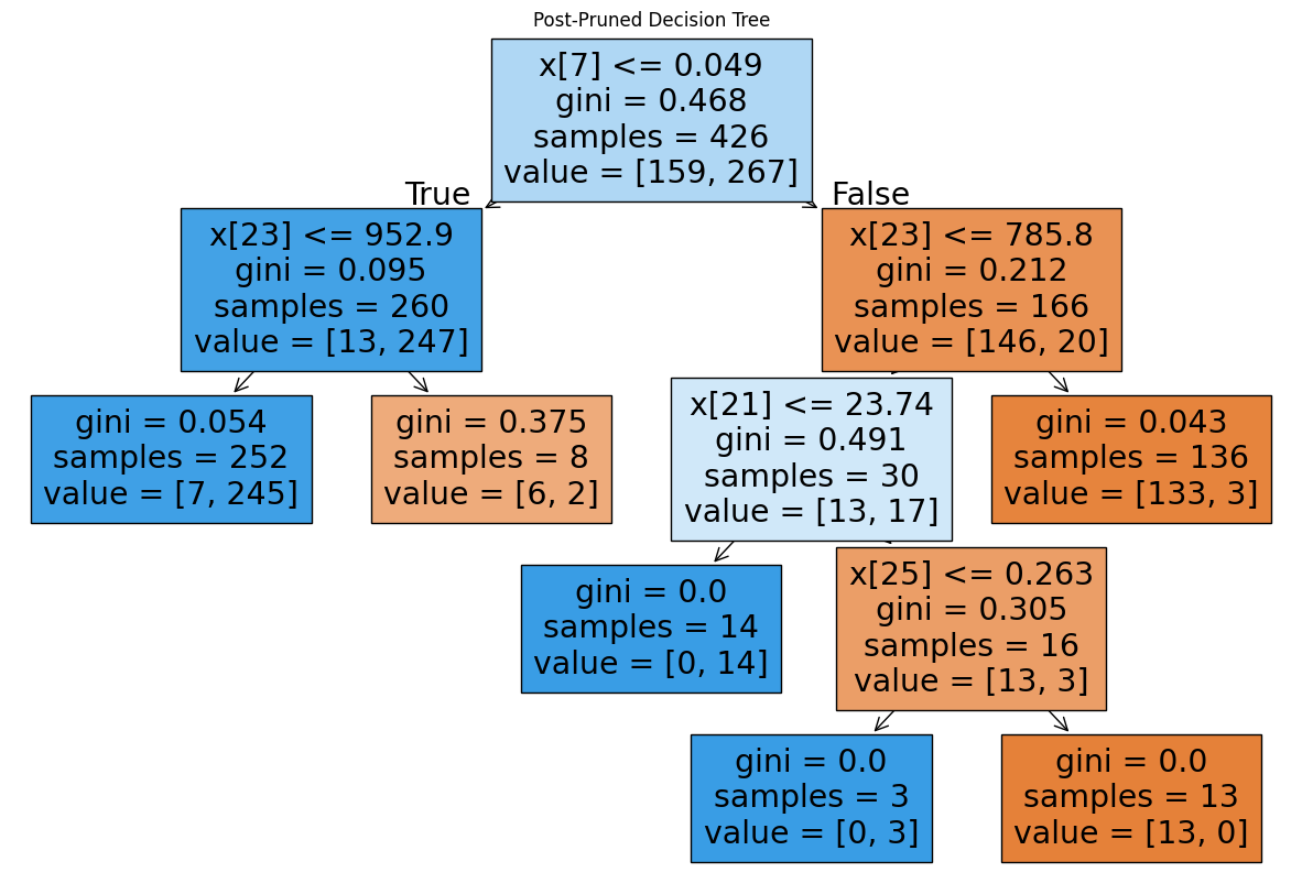
post_pruned_tree = DecisionTreeClassifier(random_state=0, ccp_alpha=0.0114)
post_pruned_tree.fit(X_train,y_train)

DecisionTreeClassifier(ccp_alpha=0.0114, random_state=0)

pred=post_pruned_tree.predict(X_test)
from sklearn.metrics import accuracy_score
print("Train Accuracy ->",post_pruned_tree.score(X_train, y_train))
print("Test Accuracy ->",accuracy_score(y_test, pred))

Train Accuracy -> 0.971830985915493
Test Accuracy -> 0.9300699300699301

from sklearn import tree
plt.figure(figsize=(15,10))

tree.plot_tree(post_pruned_tree,filled=True)
plt.title("Post-Pruned Decision Tree")

Text(0.5, 1.0, 'Post-Pruned Decision Tree')