Lasso Regression

Interactive tutorial on lasso regression with practical implementations and visualizations

Open In Colab

import matplotlib.pyplot as plt
import numpy as np
import pandas as pd
import matplotlib
from mpl_toolkits import mplot3d

from math import sqrt
SPINE_COLOR = 'gray'
import numpy as np
import matplotlib.pyplot as plt
plt.get_cmap('gnuplot2')

%matplotlib inline
# Based on: https://www.analyticsvidhya.com/blog/2016/01/complete-tutorial-ridge-lasso-regression-python/

#Define input array with angles from 60deg to 300deg converted to radians
x = np.array([i*np.pi/180 for i in range(60,300,4)])
np.random.seed(10)  #Setting seed for reproducability
y = 4*x + 7 + np.random.normal(0,3,len(x))

y_true = 4*x + 7
max_deg = 20

data_x = [x**(i+1) for i in range(max_deg)] + [y]
data_c = ['x'] + ['x_{}'.format(i+1) for i in range(1,max_deg)] + ['y']
data = pd.DataFrame(np.column_stack(data_x),columns=data_c)
data["ones"] = 1
plt.plot(data['x'],data['y'],'.', label='Data Points')
plt.plot(data['x'], y_true,'g', label='True Function')
plt.xlabel("x")
plt.ylabel("y")
plt.legend()
plt.savefig('true_function.pdf', transparent=True, bbox_inches="tight")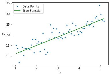

def cost(theta_0, theta_1, x, y):
    s = 0
    for i in range(len(x)):
        y_i_hat = x[i]*theta_1 + theta_0
        s += (y[i]-y_i_hat)**2
    return s/len(x)

x_grid, y_grid = np.mgrid[-4:15:.2, -4:15:.2]

cost_matrix = np.zeros_like(x_grid)
for i in range(x_grid.shape[0]):
    for j in range(x_grid.shape[1]):
        cost_matrix[i, j] = cost(x_grid[i, j], y_grid[i, j], data['x'], data['y'])

def cost_lasso(theta_0, theta_1, x, y, lamb):
    s = 0
    for i in range(len(x)):
        y_i_hat = x[i]*theta_1 + theta_0
        s += (y[i]-y_i_hat)**2 + lamb*(abs(theta_0) + abs(theta_1))
    return s/len(x)

x_grid, y_grid = np.mgrid[-4:15:.2, -4:15:.2]

#lambda  = 1000 cost curve tends to lasso objective. 
fig = plt.figure(figsize=(7,7))
lamb_list = [10,100,1000]
for lamb in lamb_list:
    lasso_cost_matrix = np.zeros_like(x_grid)
    for i in range(x_grid.shape[0]):
        for j in range(x_grid.shape[1]):
            lasso_cost_matrix[i, j] = cost_lasso(x_grid[i, j], y_grid[i, j], data['x'], data['y'],lamb)


    ax = plt.axes(projection='3d')
    ax.plot_surface(x_grid, y_grid, lasso_cost_matrix,cmap='viridis', edgecolor='none')

    ax.set_title('Least squares objective function');
    ax.set_xlabel(r"$\theta_0$")
    ax.set_ylabel(r"$\theta_1$")
    ax.set_xlim([-4,15])
    ax.set_ylim([-4,15])

    u = np.linspace(0, np.pi, 30)
    v = np.linspace(0, 2 * np.pi, 30)

    # x = np.outer(500*np.sin(u), np.sin(v))
    # y = np.outer(500*np.sin(u), np.cos(v))
    # z = np.outer(500*np.cos(u), np.ones_like(v))
    # ax.plot_wireframe(x, y, z)

    ax.view_init(45, 120)
    plt.savefig('lasso_lamb_{}_surface.pdf'.format(lamb), transparent=True, bbox_inches="tight")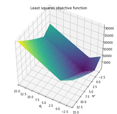

def yy(p,soln):
    xx = np.linspace(-soln,soln,100)
    xx_final = []
    yy_final = []
    for x in xx:
        if(x>0):
            xx_final.append(x)
            xx_final.append(x)
            y = (soln**p - x**p)**(1.0/p)
            yy_final.append(y)
            yy_final.append(-y)
            
        else:
            xx_final.append(x)
            xx_final.append(x)
            y = (soln**p - (-x)**p)**(1.0/p)
            yy_final.append(y)
            yy_final.append(-y)
    return xx_final, yy_final

fig,ax = plt.subplots()
ax.fill(xx_final,yy_final)

from matplotlib.patches import Rectangle

soln = 3
p  = 0.5
levels = np.sort(np.array([2,10,20,50,100,150,200,400,600,800,1000]))
fig,ax = plt.subplots()
plt.contourf(x_grid, y_grid, cost_matrix, levels,alpha=.7)
plt.colorbar()
plt.axhline(0, color='black', alpha=.5, dashes=[2, 4],linewidth=1)
plt.axvline(0, color='black', alpha=0.5, dashes=[2, 4],linewidth=1)

xx = np.linspace(-soln,soln,100)
y1  = yy1(xx,soln,p)
y2  = yy2(xx,soln,p)

x_final = np.hstack((xx,xx))
y_final = np.hstack((y1,y2))

xx_final, yy_final = yy(p,soln)

plt.fill(xx_final,yy_final)



CS = plt.contour(x_grid, y_grid, cost_matrix, levels, linewidths=1,colors='black')
plt.clabel(CS, inline=1, fontsize=8)
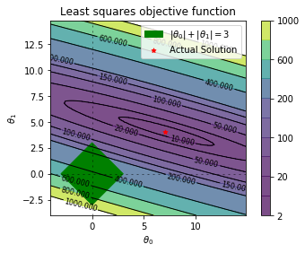
plt.title("Least squares objective function")
plt.xlabel(r"$\theta_0$")
plt.ylabel(r"$\theta_1$")
p1 = Rectangle((-soln, 0), np.sqrt(2)*soln,np.sqrt(2)*soln, angle = '-45', color='g', label=r'$|\theta_0|+|\theta_1|=3$')
plt.scatter([7], [4],marker='*', color='r',s=25,label='Actual Solution')
plt.gca().add_patch(p1)
plt.legend()
plt.gca().set_aspect('equal')

plt.savefig('lasso_base_contour.pdf', transparent=True, bbox_inches="tight")
plt.show()

from matplotlib.patches import Rectangle


levels = np.sort(np.array([2,10,20,50,100,150,200,400,600,800,1000]))
fig,ax = plt.subplots()
plt.contourf(x_grid, y_grid, cost_matrix, levels,alpha=.7)
plt.colorbar()
plt.axhline(0, color='black', alpha=.5, dashes=[2, 4],linewidth=1)
plt.axvline(0, color='black', alpha=0.5, dashes=[2, 4],linewidth=1)

plt.scatter(xx, y1, s=0.1,color='k',)
plt.scatter(xx, y2, s=0.1,color='k',)

CS = plt.contour(x_grid, y_grid, cost_matrix, levels, linewidths=1,colors='black')
plt.clabel(CS, inline=1, fontsize=8)
plt.title("Least squares objective function")
plt.xlabel(r"$\theta_0$")
plt.ylabel(r"$\theta_1$")
p1 = Rectangle((-soln, 0), np.sqrt(2)*soln,np.sqrt(2)*soln, angle = '-45', color='g', label=r'$|\theta_0|+|\theta_1|=3$')
plt.scatter([7], [4],marker='*', color='r',s=25,label='Actual Solution')
plt.gca().add_patch(p1)
plt.legend()
plt.gca().set_aspect('equal')

plt.savefig('lasso_base_contour.pdf', transparent=True, bbox_inches="tight")
plt.show()

regressor.coef_[0] + regressor.coef_[1]

5.74196012460497

## Function generator. 
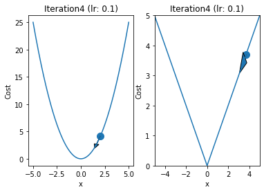
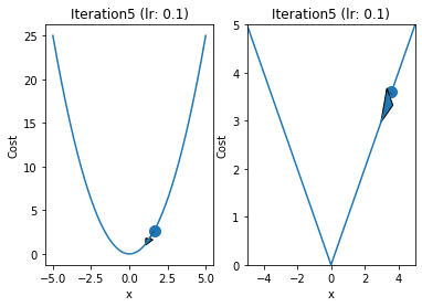
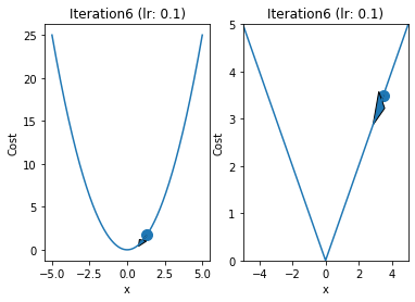
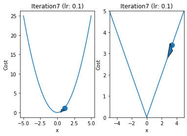
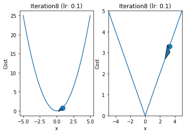
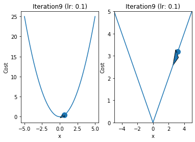
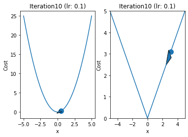
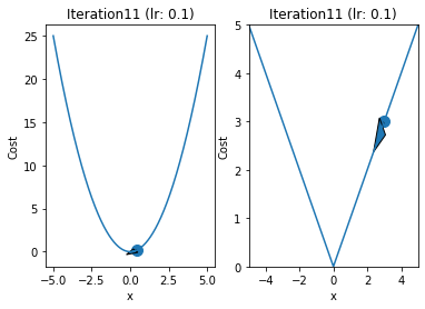
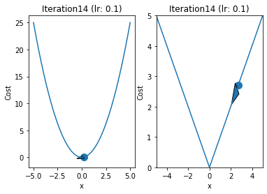
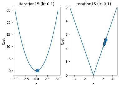
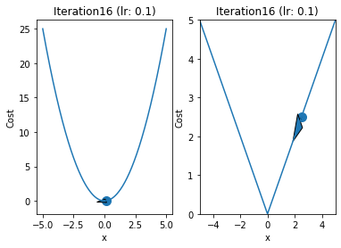
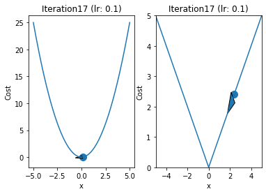
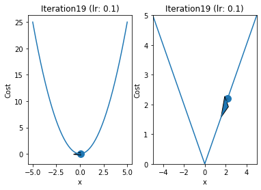
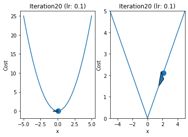
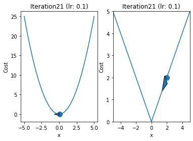
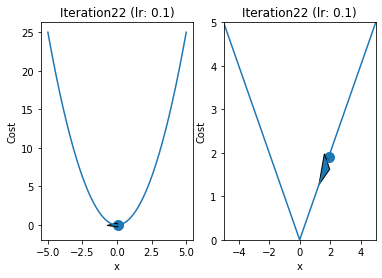
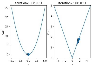
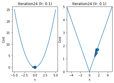
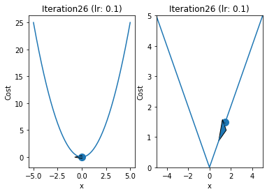
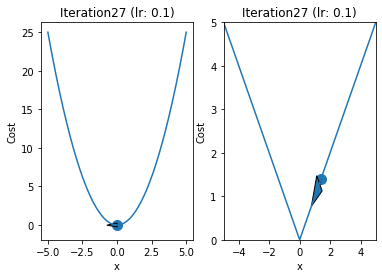
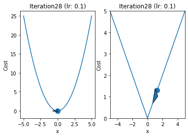
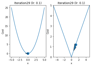
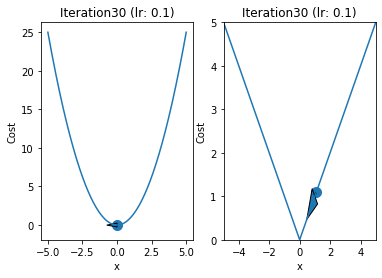
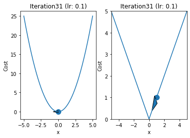
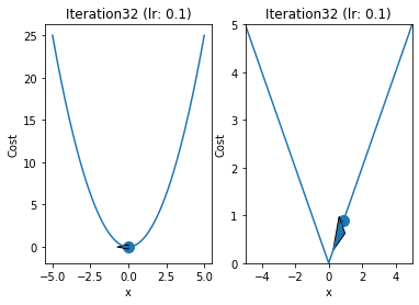
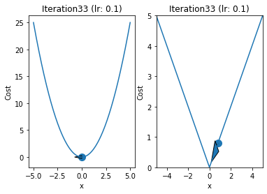
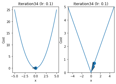
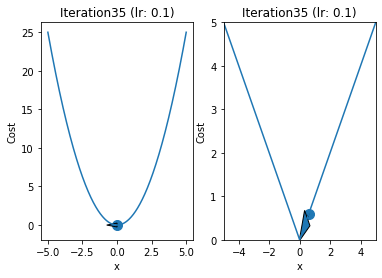
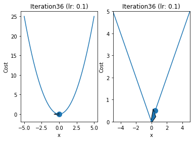
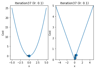
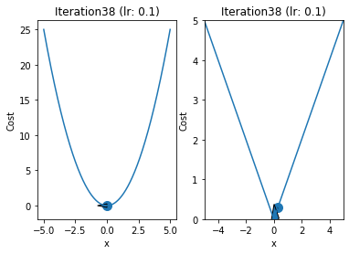
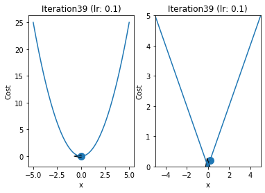
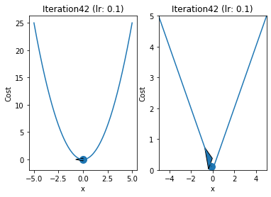
iterations = 60
p = 4
q = 4
alpha  = 0.1

x = np.linspace(-5,5,1000)
y1 = x**2
y2 = abs(x)


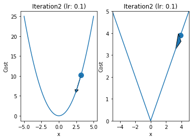
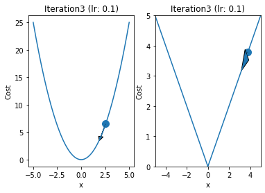
for i in range(iterations):
    fig,ax = plt.subplots(1,2)
    ax[0].plot(x,y1)
    ax[1].plot(x,y2)
    prev = p
    qrev = q
    p = p - 2*alpha*p
    q = q - alpha
    val = p
    
    ax[0].arrow(prev,prev**2,p-prev,p**2-prev**2,head_width=0.5)
    ax[1].arrow(qrev,abs(qrev),q - qrev ,abs(q) - abs(qrev),head_width = 0.5)
    ax[0].scatter([prev],[prev**2],s=100)
    ax[1].scatter([qrev],abs(qrev),s=100)
    ax[0].set_xlabel("x")
    ax[1].set_xlabel("x")
    ax[1].set_ylabel("Cost")
    ax[0].set_ylabel("Cost")
    ax[1].set_xlim(-5,5)
    ax[1].set_ylim(0,5)
    ax[1].set_title("Iteration"+str(i+1)+" (lr: "+str(alpha)+")")
    ax[0].set_title("Iteration"+str(i+1)+" (lr: "+str(alpha)+")")
    if(i==0):
        plt.savefig("GD_iteration_"+str((i+1)//10)+".pdf", format='pdf',transparent=True)
    if(i%10==9):
        plt.savefig("GD_iteration_"+str((i+1)//10)+".pdf", format='pdf',transparent=True)
    
    plt.show()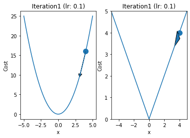

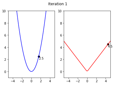
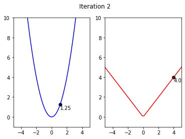
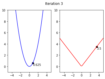
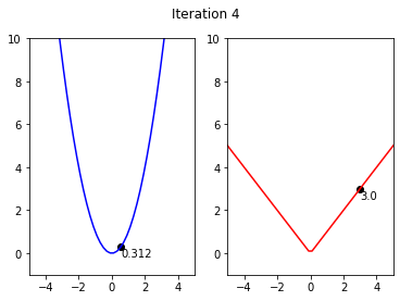
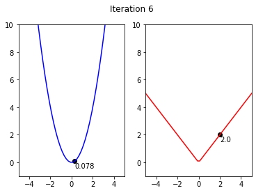
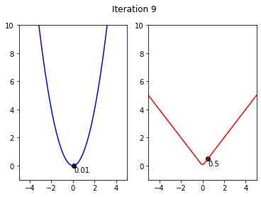
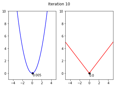
x1,y1= 5**0.5,5
y2,x2 = 5,5
x_shift = 0
y_shift = -0.5
iterations = 11
for i in range(iterations):
    fig, ax = plt.subplots(nrows=1, ncols=2)
   
    ax[0].set_ylim(-1,10)
    ax[0].set_xlim(-5,5)
    ax[1].set_xlim(-5,5)
    ax[1].set_ylim(-1,10)
    ax[0].plot(x,x**2, color = 'blue')
    ax[1].plot(x,abs(x),color = 'red')
    ax[0].scatter(x1,y1,color = 'black')
    
    ax[0].annotate(str(round(y1,3)), (x1 + x_shift, y1+y_shift))
    ax[1].annotate(str(y2), (x2 + x_shift, y2 + y_shift))
    ax[1].scatter(x2,y2,color = 'black')
    fig.suptitle('Iteration {}'.format(i))
    if(iteratio)
    plt.savefig('GD_Iteration_{}.pdf'.format(i))
    
    y1 = y1 - alpha*y1
    y2 = y2 - 0.5
    x2 = y2
    x1 = y1**0.5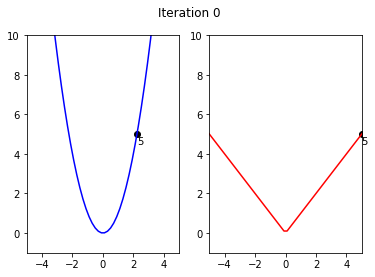

from sklearn.linear_model import Lasso
from matplotlib.patches import Rectangle


for alpha in np.linspace(1,2,5):
    fig, ax = plt.subplots(nrows=1, ncols=2, figsize=(10, 5))
    
    deg = 1
    predictors = ['ones','x']
    if deg >= 2:
        predictors.extend(['x_%d'%i for i in range(2,deg+1)])  

    regressor = Lasso(alpha=alpha,normalize=True, fit_intercept=False)
    regressor.fit(data[predictors],data['y'])
    y_pred = regressor.predict(data[predictors])

    # Plot
    ax[0].scatter(data['x'],data['y'], label='Train')
    ax[0].plot(data['x'], y_pred,'k', label='Prediction')
    ax[0].plot(data['x'], y_true,'g.', label='True Function')
    ax[0].legend() 
    ax[0].set_title(f"Degree: {deg} | $\mu$: {alpha} | Max Coef: {max(regressor.coef_, key=abs):.2f}")

    # Circle
    total = abs(regressor.coef_[0]) + abs(regressor.coef_[1])
    p1 = Rectangle((-total, 0), np.sqrt(2)*total, np.sqrt(2)*total, angle = -45, alpha=0.6, color='g', label=r'$|\theta_0|+|\theta_1|={:.2f}$'.format(total))
    ax[1].add_patch(p1)

    # Contour
    levels = np.sort(np.array([2,10,20,50,100,150,200,400,600,800,1000]))
    ax[1].contourf(x_grid, y_grid, cost_matrix, levels,alpha=.7)
    #ax[1].colorbar()
    ax[1].axhline(0, color='black', alpha=.5, dashes=[2, 4],linewidth=1)
    ax[1].axvline(0, color='black', alpha=0.5, dashes=[2, 4],linewidth=1)

    CS = plt.contour(x_grid, y_grid, cost_matrix, levels, linewidths=1,colors='black')
    ax[1].clabel(CS, inline=1, fontsize=8)
    ax[1].set_title("Least squares objective function")
    ax[1].set_xlabel(r"$\theta_0$")
    ax[1].set_ylabel(r"$\theta_1$")
    ax[1].scatter(regressor.coef_[0],regressor.coef_[1] ,marker='x', color='r',s=25,label='Lasso Solution')
    ax[1].scatter([7], [4],marker='*', color='r',s=25,label='Actual Solution')
    ax[1].set_xlim([-4,15])
    ax[1].set_ylim([-4,15])
    ax[1].legend()

    plt.savefig('lasso_{}.pdf'.format(alpha), transparent=True, bbox_inches="tight")
    plt.show()
    plt.clf()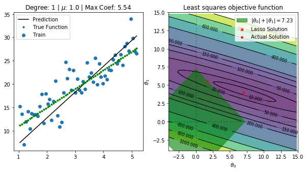

<Figure size 432x288 with 0 Axes>

<Figure size 432x288 with 0 Axes>

<Figure size 432x288 with 0 Axes>

<Figure size 432x288 with 0 Axes>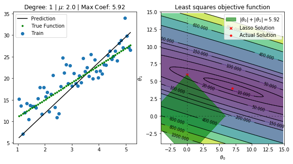

<Figure size 432x288 with 0 Axes>

from sklearn.linear_model import Lasso

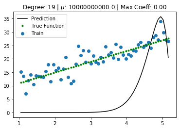
for i,deg in enumerate([19]):
    predictors = ['ones', 'x']
    if deg >= 2:
        predictors.extend(['x_%d'%i for i in range(2,deg+1)])  

    for i,alpha in enumerate([1, 1e10]):
        regressor = Lasso(alpha=alpha,normalize=False, fit_intercept=False)
        regressor.fit(data[predictors],data['y'])
        y_pred = regressor.predict(data[predictors])
        plt.scatter(data['x'],data['y'], label='Train')
        plt.plot(data['x'], y_pred,'k', label='Prediction')
        plt.plot(data['x'], y_true,'g.', label='True Function')
        plt.legend() 
        plt.title(f"Degree: {deg} | $\mu$: {alpha} | Max Coeff: {max(regressor.coef_, key=abs):.2f}")
        plt.savefig('lasso_{}_{}.pdf'.format(alpha, deg), transparent=True, bbox_inches="tight")
        plt.show()
        plt.clf()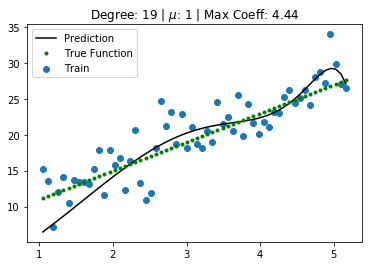

<Figure size 432x288 with 0 Axes>

import pandas as pd

data = pd.read_excel("dataset.xlsx")
cols = data.columns
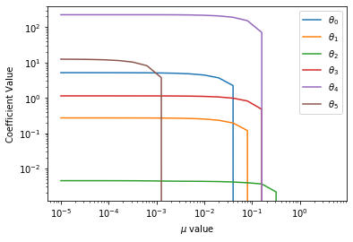
alph_list = np.logspace(-5,1,num=20, endpoint=False)
coef_list = []

for i,alpha in enumerate(alph_list):
    regressor = Lasso(alpha=alpha,normalize=True)
    regressor.fit(data[cols[1:-1]],data[cols[-1]])
    coef_list.append(regressor.coef_)

coef_list = np.abs(np.array(coef_list).T)
for i in range(len(cols[1:-1])):
    plt.loglog(alph_list, coef_list[i] , label=r"$\theta_{}$".format(i))
plt.xlabel('$\mu$ value')
plt.ylabel('Coefficient Value')
plt.legend() 
plt.savefig('lasso_reg.pdf', transparent=True, bbox_inches="tight")