import numpy as np
import matplotlib.pyplot as plt
%matplotlib inline
from latexify import *
from sklearn.linear_model import LogisticRegression
import matplotlib.patches as mpatches
%config InlineBackend.figure_format = 'retina'Logistic Regression - Basis
ML
![]()
# Choose some points betweennp.random.seed(0)
x1 = np.random.randn(1, 100)
x2 = np.random.randn(1, 100)y = x1**2 + x2**2x1array([[ 1.76405235, 0.40015721, 0.97873798, 2.2408932 , 1.86755799,
-0.97727788, 0.95008842, -0.15135721, -0.10321885, 0.4105985 ,
0.14404357, 1.45427351, 0.76103773, 0.12167502, 0.44386323,
0.33367433, 1.49407907, -0.20515826, 0.3130677 , -0.85409574,
-2.55298982, 0.6536186 , 0.8644362 , -0.74216502, 2.26975462,
-1.45436567, 0.04575852, -0.18718385, 1.53277921, 1.46935877,
0.15494743, 0.37816252, -0.88778575, -1.98079647, -0.34791215,
0.15634897, 1.23029068, 1.20237985, -0.38732682, -0.30230275,
-1.04855297, -1.42001794, -1.70627019, 1.9507754 , -0.50965218,
-0.4380743 , -1.25279536, 0.77749036, -1.61389785, -0.21274028,
-0.89546656, 0.3869025 , -0.51080514, -1.18063218, -0.02818223,
0.42833187, 0.06651722, 0.3024719 , -0.63432209, -0.36274117,
-0.67246045, -0.35955316, -0.81314628, -1.7262826 , 0.17742614,
-0.40178094, -1.63019835, 0.46278226, -0.90729836, 0.0519454 ,
0.72909056, 0.12898291, 1.13940068, -1.23482582, 0.40234164,
-0.68481009, -0.87079715, -0.57884966, -0.31155253, 0.05616534,
-1.16514984, 0.90082649, 0.46566244, -1.53624369, 1.48825219,
1.89588918, 1.17877957, -0.17992484, -1.07075262, 1.05445173,
-0.40317695, 1.22244507, 0.20827498, 0.97663904, 0.3563664 ,
0.70657317, 0.01050002, 1.78587049, 0.12691209, 0.40198936]])y[y>1] = 1
y[y<1] = 0
c = 0
for i in range(100):
if y[0, i] == 1:
y[0, i] = 0
c += 1
if c == 10:
breaklatexify()
plt.scatter(x1, x2, c=y,s=5)
yellow_patch = mpatches.Patch(color='yellow', label='Oranges')
blue_patch = mpatches.Patch(color='darkblue', label='Tomatoes')
plt.legend(handles=[yellow_patch, blue_patch])
plt.xlabel(r"$x_1$")
plt.ylabel(r"$x_2$")
plt.gca().set_aspect('equal')
format_axes(plt.gca())
plt.savefig("../figures/logistic-regression/logisitic-circular-data.pdf", bbox_inches="tight", transparent=True)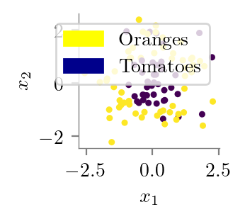
np.vstack((x1, x2)).shape(2, 100)clf_1 = LogisticRegression(penalty='none',solver='newton-cg')
clf_1.fit(np.vstack((x1, x2)).T, y.T)LogisticRegression(penalty='none', solver='newton-cg')In a Jupyter environment, please rerun this cell to show the HTML representation or trust the notebook.
On GitHub, the HTML representation is unable to render, please try loading this page with nbviewer.org.
LogisticRegression(penalty='none', solver='newton-cg')
X = np.vstack((x1, x2)).T
# create a mesh to plot in
x_min, x_max = X[:, 0].min() - 0.3, X[:, 0].max() + 0.3
y_min, y_max = X[:, 1].min() - 0.3, X[:, 1].max() + 0.3
h = 0.02
xx, yy = np.meshgrid(np.arange(x_min, x_max, h),
                     np.arange(y_min, y_max, h))


Z = clf_1.predict(np.c_[xx.ravel(), yy.ravel()])

# Put the result into a color plot
Z = Z.reshape(xx.shape)
latexify()
yellow_patch = mpatches.Patch(color='yellow', label='Oranges')
blue_patch = mpatches.Patch(color='darkblue', label='Tomatoes')
pink_patch = mpatches.Patch(color='darksalmon', label='Predict oranges')
lblue_patch = mpatches.Patch(color='lightblue', label='Predict tomatoes')
plt.legend(handles=[yellow_patch, blue_patch, pink_patch, lblue_patch], loc='upper center',
           bbox_to_anchor=(0.5, 1.25),
          ncol=2, fancybox=True, shadow=True)

plt.contourf(xx, yy, Z, cmap=plt.cm.Paired, alpha=0.4)
plt.gca().set_aspect('equal')
plt.scatter(x1, x2, c=y,s=5)
plt.xlabel(r"$x_1$")
plt.ylabel(r"$x_2$")
plt.gca().set_aspect('equal')
plt.savefig("../figures/logistic-regression/logisitic-linear-prediction.pdf", bbox_inches="tight", transparent=True)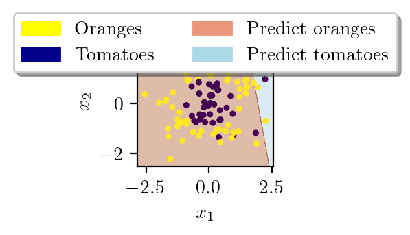
new_x = np.zeros((4, 100))new_x[0] = x1
new_x[1] = x2
new_x[2] = x1**2
new_x[3] = x2**2clf = LogisticRegression(penalty='none',solver='newton-cg')clf.fit(new_x.T, y.T)LogisticRegression(penalty='none', solver='newton-cg')In a Jupyter environment, please rerun this cell to show the HTML representation or trust the notebook.
On GitHub, the HTML representation is unable to render, please try loading this page with nbviewer.org.
LogisticRegression(penalty='none', solver='newton-cg')
clf.coef_array([[-0.50464855, -0.30337009, 1.08937351, 0.73697949]])new_x.T[:, 0]array([ 1.76405235, 0.40015721, 0.97873798, 2.2408932 , 1.86755799,
-0.97727788, 0.95008842, -0.15135721, -0.10321885, 0.4105985 ,
0.14404357, 1.45427351, 0.76103773, 0.12167502, 0.44386323,
0.33367433, 1.49407907, -0.20515826, 0.3130677 , -0.85409574,
-2.55298982, 0.6536186 , 0.8644362 , -0.74216502, 2.26975462,
-1.45436567, 0.04575852, -0.18718385, 1.53277921, 1.46935877,
0.15494743, 0.37816252, -0.88778575, -1.98079647, -0.34791215,
0.15634897, 1.23029068, 1.20237985, -0.38732682, -0.30230275,
-1.04855297, -1.42001794, -1.70627019, 1.9507754 , -0.50965218,
-0.4380743 , -1.25279536, 0.77749036, -1.61389785, -0.21274028,
-0.89546656, 0.3869025 , -0.51080514, -1.18063218, -0.02818223,
0.42833187, 0.06651722, 0.3024719 , -0.63432209, -0.36274117,
-0.67246045, -0.35955316, -0.81314628, -1.7262826 , 0.17742614,
-0.40178094, -1.63019835, 0.46278226, -0.90729836, 0.0519454 ,
0.72909056, 0.12898291, 1.13940068, -1.23482582, 0.40234164,
-0.68481009, -0.87079715, -0.57884966, -0.31155253, 0.05616534,
-1.16514984, 0.90082649, 0.46566244, -1.53624369, 1.48825219,
1.89588918, 1.17877957, -0.17992484, -1.07075262, 1.05445173,
-0.40317695, 1.22244507, 0.20827498, 0.97663904, 0.3563664 ,
0.70657317, 0.01050002, 1.78587049, 0.12691209, 0.40198936])X = np.vstack((x1, x2)).T
X.shape(100, 2)# create a mesh to plot in
x_min, x_max = X[:, 0].min() - 0.3, X[:, 0].max() + 0.3
y_min, y_max = X[:, 1].min() - 0.3, X[:, 1].max() + 0.3
h = 0.02
xx, yy = np.meshgrid(np.arange(x_min, x_max, h),
np.arange(y_min, y_max, h))
Z = clf.predict(np.c_[xx.ravel(), yy.ravel(), np.square(xx.ravel()), np.square(yy.ravel())])
# Put the result into a color plot
Z = Z.reshape(xx.shape)
latexify()
yellow_patch = mpatches.Patch(color='yellow', label='Oranges')
blue_patch = mpatches.Patch(color='darkblue', label='Tomatoes')
pink_patch = mpatches.Patch(color='darksalmon', label='Predict oranges')
lblue_patch = mpatches.Patch(color='lightblue', label='Predict tomatoes')
plt.legend(handles=[yellow_patch, blue_patch, pink_patch, lblue_patch], loc='upper center',
bbox_to_anchor=(0.5, 1.25),
ncol=2, fancybox=True, shadow=True)
plt.contourf(xx, yy, Z, cmap=plt.cm.Paired, alpha=0.4)
plt.gca().set_aspect('equal')
plt.scatter(x1, x2, c=y,s=5)
plt.xlabel(r"$x_1$")
plt.ylabel(r"$x_2$")
plt.gca().set_aspect('equal')
plt.savefig("../figures/logistic-regression/logisitic-circular-prediction.pdf", bbox_inches="tight", transparent=True)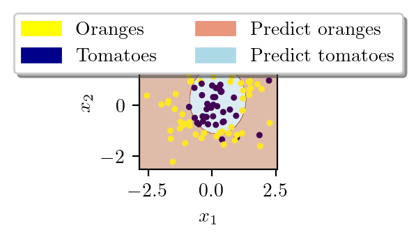
Z.shape(261, 272)np.c_[xx.ravel(), yy.ravel(), np.square(xx.ravel()), np.square(yy.ravel())]array([[-2.85298982, -2.52340315, 8.13955089, 6.36756347],
[-2.83298982, -2.52340315, 8.0258313 , 6.36756347],
[-2.81298982, -2.52340315, 7.9129117 , 6.36756347],
...,
[ 2.52701018, 2.67659685, 6.38578047, 7.16417069],
[ 2.54701018, 2.67659685, 6.48726088, 7.16417069],
[ 2.56701018, 2.67659685, 6.58954129, 7.16417069]])xx.ravel()array([-2.85298982, -2.83298982, -2.81298982, ..., 2.52701018,
2.54701018, 2.56701018])# create a mesh to plot in
x_min, x_max = X[:, 0].min() - h, X[:, 0].max() + h
y_min, y_max = X[:, 1].min() - h, X[:, 1].max() + h
h = 0.02
xx, yy = np.meshgrid(np.arange(x_min, x_max, h),
np.arange(y_min, y_max, h))
Z = clf.predict_proba(np.c_[xx.ravel(), yy.ravel(), np.square(xx.ravel()), np.square(yy.ravel())])
# Put the result into a color plot
Z = Z[:, 0].reshape(xx.shape)
latexify()
plt.contourf(xx, yy, Z,levels=np.linspace(0, 1.1, num=10),cmap='Blues')
plt.gca().set_aspect('equal')
#plt.scatter(x1, x2, c=y)
plt.xlabel(r"$x_1$")
plt.ylabel(r"$x_2$")
plt.colorbar(label='P(Tomatoes)')
plt.savefig("../figures/logistic-regression/logisitic-circular-probability.pdf", bbox_inches="tight", transparent=True)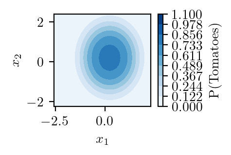
xx.shape(233, 244)Z.size56852np.linspace(0, 1.1, num=50)array([0. , 0.02244898, 0.04489796, 0.06734694, 0.08979592,
0.1122449 , 0.13469388, 0.15714286, 0.17959184, 0.20204082,
0.2244898 , 0.24693878, 0.26938776, 0.29183673, 0.31428571,
0.33673469, 0.35918367, 0.38163265, 0.40408163, 0.42653061,
0.44897959, 0.47142857, 0.49387755, 0.51632653, 0.53877551,
0.56122449, 0.58367347, 0.60612245, 0.62857143, 0.65102041,
0.67346939, 0.69591837, 0.71836735, 0.74081633, 0.76326531,
0.78571429, 0.80816327, 0.83061224, 0.85306122, 0.8755102 ,
0.89795918, 0.92040816, 0.94285714, 0.96530612, 0.9877551 ,
1.01020408, 1.03265306, 1.05510204, 1.07755102, 1.1 ])