Logistic Regression - Cost Function

Author

Nipun Batra

Published

January 1, 2024

Open In Colab

import numpy as np
import matplotlib.pyplot as plt
%matplotlib inline
from latexify import *
# Matplotlib retina
%config InlineBackend.figure_format = 'retina'

X = np.array([
    [1],
    [2],
    [3],
    [4],
    [5],
    [6]
])

y = np.array([1, 1, 1, 0, 0, 0])

from sklearn.linear_model import LogisticRegression

lr = LogisticRegression(penalty='none',solver='newton-cg')

lr.fit(X, y)

LogisticRegression(penalty='none', solver='newton-cg')

In a Jupyter environment, please rerun this cell to show the HTML representation or trust the notebook.
On GitHub, the HTML representation is unable to render, please try loading this page with nbviewer.org.

lr.coef_

array([[-18.33148189]])

lr.intercept_

array([64.11147504])

def sigmoid(z):
    return 1/(1+np.exp(z))

theta_0_li, theta_1_li = np.meshgrid(np.linspace(-10, 10, 200), np.linspace(-10, 10, 200))

def cost_rmse(theta_0, theta_1):
    y_hat = sigmoid(theta_0 + theta_1*X)
    err = np.sum((y-y_hat)**2)
    return err

z = np.zeros((len(theta_0_li), len(theta_0_li)))
for i in range(len(theta_0_li)):
    for j in range(len(theta_0_li)):
        z[i, j] = cost_rmse(theta_0_li[i, j], theta_1_li[i, j])

latexify()
plt.contourf(theta_0_li, theta_1_li, z)
plt.xlabel(r'$\theta_0$')
plt.ylabel(r'$\theta_1$')
plt.colorbar()
plt.title('RMSE contour plot')
format_axes(plt.gca())
plt.savefig("../figures/logistic-regression/logistic-sse-loss-contour.pdf", bbox_inches="tight", transparent=True)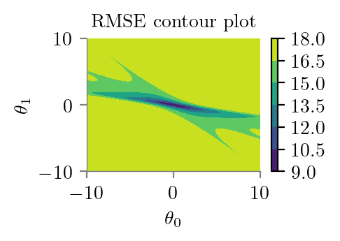

import matplotlib.pyplot as plt
from mpl_toolkits.mplot3d import Axes3D
latexify()
fig = plt.figure()
ax = fig.add_subplot(111, projection='3d')
ax.plot_surface(theta_0_li, theta_1_li, z)
ax.set_title('RMSE surface plot')
ax.set_xlabel(r'$\theta_0$')
ax.set_ylabel(r'$\theta_1$')
plt.tight_layout()
plt.savefig("../figures/logistic-regression/logistic-sse-loss-3d.pdf", bbox_inches="tight", transparent=True)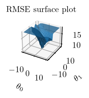

import pandas as pd

pd.DataFrame(z).min().min()

9.01794626038055

def cost_2(theta_0, theta_1):
    y_hat = sigmoid(theta_0 + theta_1*X)
    
    err = -np.sum((y*np.log(y_hat) + (1-y)*np.log(1-y_hat)))
    return err

z2 = np.zeros((len(theta_0_li), len(theta_0_li)))
for i in range(len(theta_0_li)):
    for j in range(len(theta_0_li)):
        z2[i, j] = cost_2(theta_0_li[i, j], theta_1_li[i, j])

import matplotlib.pyplot as plt
from mpl_toolkits.mplot3d import Axes3D

latexify()
fig = plt.figure()
ax = fig.add_subplot(111, projection='3d')
ax.plot_surface(theta_0_li, theta_1_li, z2)
ax.set_title('Cross-entropy surface plot')
ax.set_xlabel(r'$\theta_0$')
ax.set_ylabel(r'$\theta_1$')
plt.tight_layout()
plt.savefig("../figures/logistic-regression/logistic-cross-loss-surface.pdf", bbox_inches="tight", transparent=True)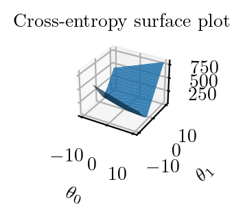

latexify()
plt.contourf(theta_0_li, theta_1_li, z2)
plt.title('Cross-entropy contour plot')
plt.colorbar()
plt.xlabel(r'$\theta_0$')
plt.ylabel(r'$\theta_1$')
format_axes(plt.gca())
plt.savefig("../figures/logistic-regression/logistic-cross-loss-contour.pdf", bbox_inches="tight", transparent=True)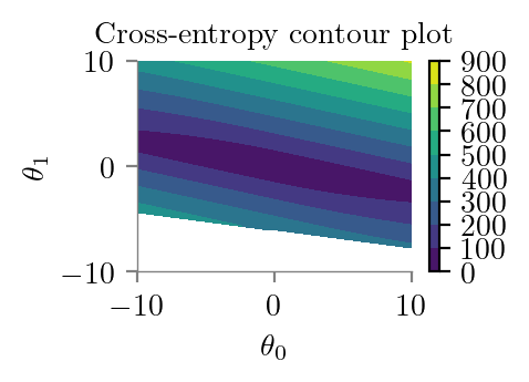

y.shape, y_bar.shape

((6,), (10000,))

y = 0
y_bar = np.linspace(0, 1.1, 10000)
plt.plot(y_bar, -y*np.log(y_bar) - (1-y)*np.log(1-y_bar))
format_axes(plt.gca())
plt.ylabel("Cost when y = 0")
plt.xlabel(r'$\hat{y}$')
plt.savefig("../figures/logistic-regression/logistic-cross-cost-0.pdf", bbox_inches="tight", transparent=True)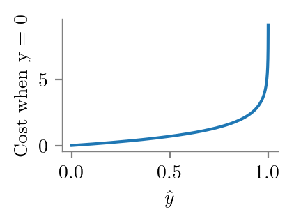

y = 1
y_bar = np.linspace(0, 1.1, 10000)
plt.plot(y_bar, -y*np.log(y_bar) - (1-y)*np.log(1-y_bar))
format_axes(plt.gca())
plt.ylabel("Cost when y = 1")
plt.xlabel(r'$\hat{y}$')
plt.savefig("../figures/logistic-regression/logistic-cross-cost-1.pdf", bbox_inches="tight", transparent=True)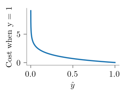

Likelihood

X_with_one = np.hstack((np.ones_like(X), X))

\[\begin{align*} P(y | X, \theta) &= \prod_{i=1}^{n} P(y_{i} | x_{i}, \theta) \\ &= \prod_{i=1}^{n} \Big\{\frac{1}{1 + e^{-x_{i}^{T}\theta}}\Big\}^{y_{i}}\Big\{1 - \frac{1}{1 + e^{-x_{i}^{T}\theta}}\Big\}^{1 - y_{i}} \\ \end{align*}\]

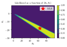
X_with_one[1]

array([1, 2])

def likelihood(theta_0, theta_1):
    s = 1

    for i in range(len(X)):
        y_i_hat = sigmoid(-X_with_one[i]@np.array([theta_0, theta_1]))
        s = s* ((y_i_hat**y[i])*(1-y_i_hat)**(1-y[i]))
    
    
    return s

x_grid_2, y_grid_2 = np.mgrid[-5:100:0.5, -30:10:.1]

li = np.zeros_like(x_grid_2)
for i in range(x_grid_2.shape[0]):
    for j in range(x_grid_2.shape[1]):
        li[i, j] = likelihood(x_grid_2[i, j], y_grid_2[i, j])

plt.contourf(x_grid_2, y_grid_2, li)
#plt.gca().set_aspect('equal')
plt.xlabel(r"$\theta_0$")
plt.ylabel(r"$\theta_1$")
plt.colorbar()
plt.scatter(lr.intercept_[0], lr.coef_[0], s=200, marker='*', color='r', label='MLE')
plt.title(r"Likelihood as a function of ($\theta_0, \theta_1$)")
#plt.gca().set_aspect('equal')
plt.legend()
plt.savefig("../figures/logistic-regression/logistic-likelihood.pdf", bbox_inches="tight", transparent=True)