import numpy as np
import matplotlib.pyplot as plt
plt.get_cmap('gnuplot2')Maths For Ml 2
Interactive tutorial on maths for ml 2 with practical implementations and visualizations
![]()
xlist = np.linspace(-5.0, 5.0, 100)
ylist = np.linspace(-5.0, 5.0, 100)
X, Y = np.meshgrid(xlist, ylist)
Z = np.sqrt(X**2 + Y**2)
fig,ax=plt.subplots(1,1)
cp = ax.contour(X, Y, Z)

ax.clabel(cp, inline=1, fontsize=10)
# fig.colorbar(cp) # Add a colorbar to a plot
ax.set_title('Filled Contours Plot')
#ax.set_xlabel('x (cm)')
# ax.set_ylabel('y (cm)')
plt.savefig("contour-plot-1.eps", format='eps',transparent=True)
plt.show()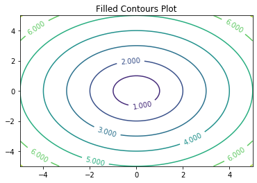
xlist = np.linspace(-5.0, 5.0, 100)
ylist = np.linspace(-5.0, 5.0, 100)
X, Y = np.meshgrid(xlist, ylist)
Z = np.sqrt(X**2)
fig,ax=plt.subplots(1,1)
cp = ax.contour(X, Y, Z)

ax.clabel(cp, inline=1, fontsize=10)
# fig.colorbar(cp) # Add a colorbar to a plot
ax.set_title('Contour Plot')
#ax.set_xlabel('x (cm)')
# ax.set_ylabel('y (cm)')
plt.savefig("contour-plot-2.eps", format='eps',transparent=True)
plt.show()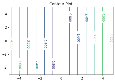
xlist = np.linspace(-5.0, 5.0, 100)
ylist = np.linspace(-5.0, 5.0, 100)
X, Y = np.meshgrid(xlist, ylist)
Z = np.sqrt(np.abs(X) + np.abs(Y))
fig,ax=plt.subplots(1,1)
cp = ax.contour(X, Y, Z)

ax.clabel(cp, inline=1, fontsize=10)
# fig.colorbar(cp) # Add a colorbar to a plot
ax.set_title('Contour Plot')
#ax.set_xlabel('x (cm)')
# ax.set_ylabel('y (cm)')
plt.savefig("contour-plot-3.eps", format='eps',transparent=True)
plt.show()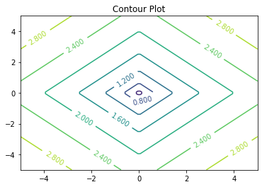
xlist = np.linspace(-5.0, 5.0, 100)
ylist = np.linspace(-2.0, 8.0, 100)
X, Y = np.meshgrid(xlist, ylist)
Z = np.sqrt(Y*(X**2))
fig,ax=plt.subplots(1,1)
cp = ax.contour(X, Y, Z)

ax.clabel(cp, inline=1, fontsize=10)
# fig.colorbar(cp) # Add a colorbar to a plot
ax.set_title('Contour Plot')
#ax.set_xlabel('x (cm)')
# ax.set_ylabel('y (cm)')
plt.savefig("contour-plot-4.eps", format='eps',transparent=True)
plt.show()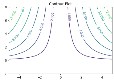
xlist = np.linspace(-5.0, 5.0, 100)
ylist = np.linspace(-5.0, 5.0, 100)
X, Y = np.meshgrid(xlist, ylist)
Z = np.sqrt(X*Y)
fig,ax=plt.subplots(1,1)
cp = ax.contour(X, Y, Z)

ax.clabel(cp, inline=1, fontsize=10)
# fig.colorbar(cp) # Add a colorbar to a plot
ax.set_title('Contour Plot')
#ax.set_xlabel('x (cm)')
# ax.set_ylabel('y (cm)')
plt.savefig("contour-plot-5.eps", format='eps',transparent=True)
plt.show()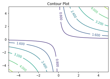
from matplotlib.pyplot import cm
import numpy as np
import matplotlib.pyplot as plt
plt.figure(figsize=(10,10))
# Contour Plot
X, Y = np.mgrid[-1:1:100j, -1:1:100j]
Z = X**2 + Y**2
cp = plt.contour(X, Y, Z)
# cb = plt.colorbar(cp)

# Vector Field
Y, X = np.mgrid[-1:1:30j, -1:1:30j]
U = 2*X
V = 2*Y
speed = np.sqrt(U**2 + V**2)
UN = U/speed
VN = V/speed
quiv = plt.quiver(X, Y, UN, VN,  # assign to var
           color='Teal',
           headlength=7)
plt.savefig("gradient-field.eps", format='eps',transparent=True)
plt.show()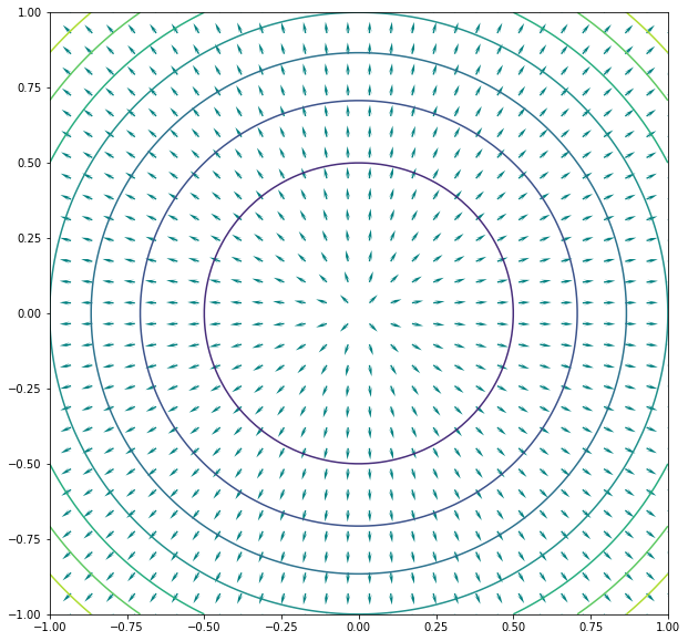
xlist = np.linspace(-5.0, 5.0, 100)
ylist = np.linspace(-5.0, 5.0, 100)
X, Y = np.meshgrid(xlist, ylist)
Z = np.sqrt(X**2+ Y**2)

fig, ax=plt.subplots(1,1,figsize=(4,4))
cp = ax.contour(X, Y, Z,levels=[1,2,3,4,5,6,7,8,9])

ax.clabel(cp, inline=1, fontsize=10)
# fig.colorbar(cp) # Add a colorbar to a plot
ax.set_title('Contour Plot')
#ax.set_xlabel('x (cm)')
# ax.set_ylabel('y (cm)')

d = np.linspace(0.11,4.5,600)
plt.plot(d,0.5/d)
# ax.arrow(1.13 , 1/1.13**2, 0, 0, head_width=0.05, head_length=0.1, fc='k', ec='k')
plt.savefig("contour-plot-6.eps", format='eps',transparent=True)
plt.show()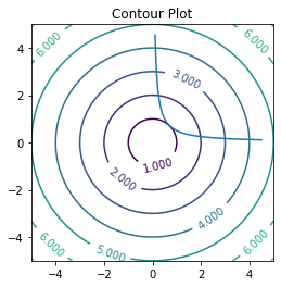
for i in np.linspace(0,2,100):
    print (i,0.5 - i**2 + 1/i**2)
0.0 inf
0.020202020202020204 2450.7495918783793
0.04040404040404041 613.0608675135189
0.06060606060606061 272.74632690541773
0.08080808080808081 153.63409505407608
0.10101010101010102 98.4997969594939
0.12121212121212122 68.54780762167124
0.14141414141414144 50.4851040814244
0.16161616161616163 38.75903646630445
0.18181818181818182 30.71694214876033
0.20202020202020204 24.96168783797571
0.22222222222222224 20.700617283950617
0.24242424242424243 17.45685548668503
0.26262626262626265 14.929548156238129
0.2828282828282829 12.92128367263648
0.30303030303030304 11.298172635445361
0.32323232323232326 9.966809927717833
0.3434343434343435 8.860426554171964
0.36363636363636365 7.930268595041323
0.38383838383838387 7.1400642169759925
0.4040404040404041 6.462376351902866
0.42424242424242425 5.876140814452502
0.4444444444444445 5.364969135802469
0.4646464646464647 4.9159562148764175
0.48484848484848486 4.518828196740127
0.5050505050505051 4.165323987348229
0.5252525252525253 3.848739962230637
0.5454545454545455 3.5635904499540856
0.5656565656565657 3.305351527280638
0.5858585858585859 3.0702655556635308
0.6060606060606061 2.8551905417814507
0.6262626262626263 2.65748294812874
0.6464646464646465 2.474905726496339
0.6666666666666667 2.305555555555555
0.686868686868687 2.1478048326048214
0.7070707070707072 2.0002550968351827
0.7272727272727273 1.8616993801652892
0.7474747474747475 1.7310915822381832
0.7676767676767677 1.6075214108402638
0.787878787878788 1.4901937611727818
0.8080808080808082 1.3784116576114678
0.8282828282828284 1.27156207154134
0.8484848484848485 1.1691040741365415
0.8686868686868687 1.0705588948578604
0.888888888888889 0.9755015432098765
0.9090909090909092 0.8835537190082641
0.9292929292929294 0.7943777895623855
0.9494949494949496 0.7076716541475031
0.9696969696969697 0.6231643494605139
0.98989898989899 0.5406122763442311
1.0101010101010102 0.4597959493929188
1.0303030303030305 0.3805171882397417
1.0505050505050506 0.302596683242079
1.0707070707070707 0.22587187959584054
1.090909090909091 0.15019513314967814
1.1111111111111112 0.07543209876543189
1.1313131313131315 0.0014603183062319447
1.1515151515151516 -0.07183201951522311
1.1717171717171717 -0.14454717092494984
1.191919191919192 -0.2167788004559923
1.2121212121212122 -0.2886128328741967
1.2323232323232325 -0.36012820815496915
1.2525252525252526 -0.4313975519179223
1.272727272727273 -0.5024877719682923
1.292929292929293 -0.5734605901083917
1.3131313131313131 -0.6443730171236
1.3333333333333335 -0.7152777777777782
1.3535353535353536 -0.7862236917418948
1.373737373737374 -0.8572560156014735
1.393939393939394 -0.9284167504222499
1.4141414141414144 -0.9997449187817161
1.4343434343434345 -1.0712768146824043
1.4545454545454546 -1.143046229338843
1.474747474747475 -1.2150846554637709
1.494949494949495 -1.2874214723620951
1.5151515151515154 -1.3600841138659328
1.5353535353535355 -1.4330982209048717
1.5555555555555556 -1.5064877802973042
1.575757575757576 -1.58027525116686
1.595959595959596 -1.6544816802290594
1.6161616161616164 -1.729126807054128
1.6363636363636365 -1.8042291602897669
1.6565656565656568 -1.8798061457204203
1.676767676767677 -1.9558741269450486
1.696969696969697 -2.032448499372201
1.7171717171717173 -2.1095437581575784
1.7373737373737375 -2.187173560644274
1.7575757575757578 -2.2653507838082487
1.777777777777778 -2.344087577160494
1.7979797979797982 -2.423395411511965
1.8181818181818183 -2.503285123966943
1.8383838383838385 -2.583766959474586
1.8585858585858588 -2.664850609236279
1.878787878787879 -2.7465452462378015
1.8989898989898992 -2.828859558149688
1.9191919191919193 -2.9118017778162164
1.9393939393939394 -2.9953797115329435
1.9595959595959598 -3.079600765294187
1.97979797979798 -3.1644719691753447
2.0 -3.25xlist = np.linspace(-2.0, 2.0, 100)
ylist = np.linspace(-2.0, 2.0, 100)
X, Y = np.meshgrid(xlist, ylist)
Z = np.sqrt(X**2+ Y**2)
fig, ax=plt.subplots(1,1,figsize=(4,4))
contours = ax.contour(X, Y, Z,levels=[0.1,0.2,.3,.4,.5,.6,.7,.8,.9,1])#,levels=[.5**(.5),2,3,4,5,6,7,8,9])
plt.clabel(contours, inline=True, fontsize=8)
ax.clabel(cp, inline=1, fontsize=10)
# fig.colorbar(cp) # Add a colorbar to a plot
ax.set_title('Contour Plot')
#ax.set_xlabel('x (cm)')
# ax.set_ylabel('y (cm)')
d = np.linspace(-4,5,600)
plt.plot(d,1-d)
plt.xlim(-1,1)
plt.ylim(-1,1)
# ax.arrow(1.13 , 1/1.13**2, 0, 0, head_width=0.05, head_length=0.1, fc='k', ec='k')
plt.savefig("contour-plot-7.eps", format='eps',transparent=True)
plt.show()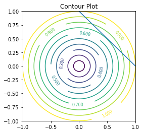
(2*0.5**2)**(.5)0.7071067811865476