Ridge

Interactive tutorial on ridge with practical implementations and visualizations

Open In Colab

import matplotlib.pyplot as plt
import numpy as np
import pandas as pd
import matplotlib

from latexify import latexify, format_axes

latexify()

#Define input array with angles from 60deg to 300deg converted to radians
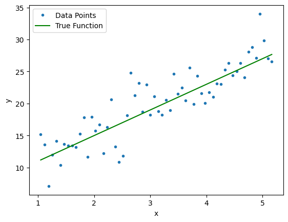
x = np.array([i*np.pi/180 for i in range(60,300,4)])
np.random.seed(10)  #Setting seed for reproducability
y = 4*x + 7 + np.random.normal(0,3,len(x))
y_true = 4*x + 7
max_deg = 20
data_x = [x**(i+1) for i in range(max_deg)] + [y]
data_c = ['x'] + ['x_{}'.format(i+1) for i in range(1,max_deg)] + ['y']
data = pd.DataFrame(np.column_stack(data_x),columns=data_c)
data["ones"] = 1
plt.plot(data['x'],data['y'],'.', label='Data Points')
plt.plot(data['x'], y_true,'g', label='True Function')
plt.xlabel("x")
plt.ylabel("y")
plt.legend()
format_axes(plt.gca())
plt.savefig('lin_1.pdf', transparent=True, bbox_inches="tight")

---------------------------------------------------------------------------
NameError                                 Traceback (most recent call last)
Cell In[2], line 16
     14 plt.ylabel("y")
     15 plt.legend()
---> 16 format_axes(plt.gca())
     17 plt.savefig('lin_1.pdf', transparent=True, bbox_inches="tight")

NameError: name 'format_axes' is not defined

from sklearn.preprocessing import PolynomialFeatures
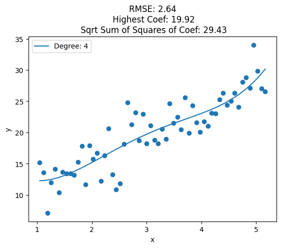
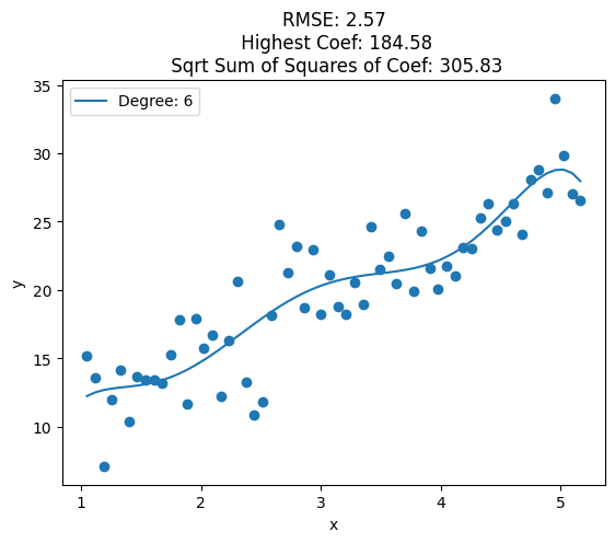
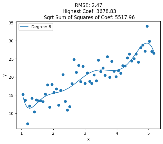
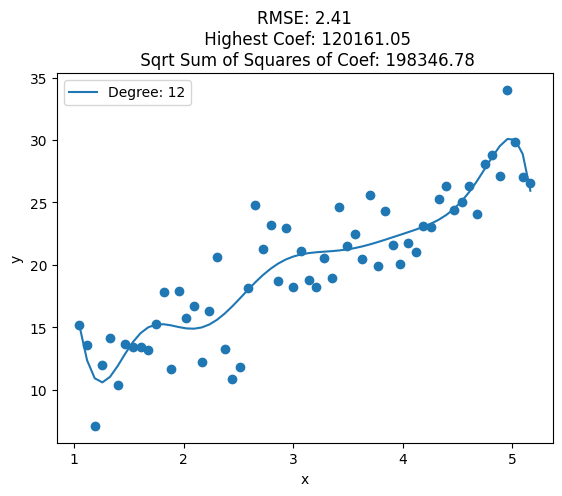
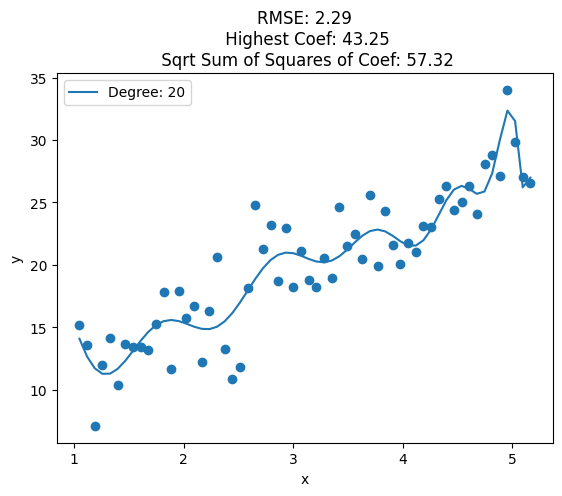
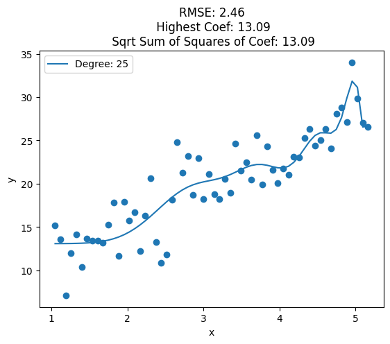
for i, deg in enumerate([1, 2, 3, 4, 5, 6, 7, 8, 10, 12, 15, 20, 25]):
    poly = PolynomialFeatures(degree=deg, include_bias=False)
    X_ = poly.fit_transform(x.reshape(-1, 1))
    from sklearn.linear_model import LinearRegression
    clf = LinearRegression()
    clf.fit(X_, data['y'])
    print(X_.shape)
    y_pred = clf.predict(X_)
    plt.figure()
    plt.plot(data['x'], y_pred, label='Degree: {}'.format(deg))
    plt.xlabel("x")
    plt.ylabel("y")
    plt.scatter(x, y)
    plt.legend()
    train_rmse = np.sqrt(np.mean((y_pred - y)**2))
    highest_coef = np.max([np.max(clf.coef_), clf.intercept_])
    sqrt_sum_squares_coef = np.sqrt(np.sum(clf.coef_**2) + clf.intercept_**2)
    plt.title('RMSE: {:.2f}\n Highest Coef: {:.2f}\n Sqrt Sum of Squares of Coef: {:.2f}'.format(train_rmse, highest_coef, sqrt_sum_squares_coef))
    #format_axes(plt.gca())
    #plt.savefig('lin_{}.pdf'.format(i+2), transparent=True, bbox_inches="tight")

(60, 1)
(60, 2)
(60, 3)
(60, 4)
(60, 5)
(60, 6)
(60, 7)
(60, 8)
(60, 10)
(60, 12)
(60, 15)
(60, 20)
(60, 25)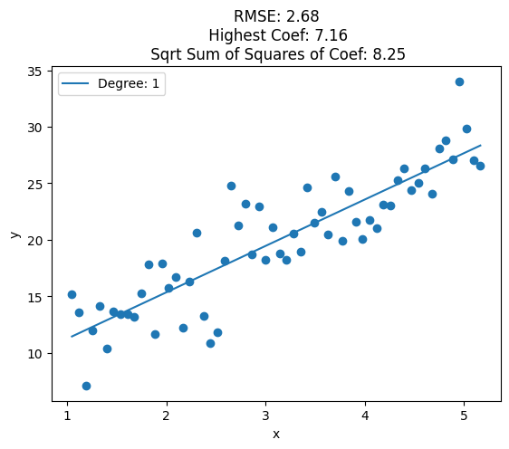

from sklearn.linear_model import LinearRegression
coef_list = []
for i,deg in enumerate([1,3,6,11]):
    predictors = ['ones','x']
    if deg >= 2:
        predictors.extend(['x_%d'%i for i in range(2,deg+1)])  

    regressor = LinearRegression(normalize=False, fit_intercept=False)  
    regressor.fit(data[predictors],data['y'])
    y_pred = regressor.predict(data[predictors])
    coef_list.append(abs(max(regressor.coef_, key=abs)))

    plt.scatter(data['x'],data['y'], label='Train')
    plt.plot(data['x'], y_pred,'k', label='Prediction')
    plt.plot(data['x'], y_true,'g.', label='True Function')
    format_axes(plt.gca())
    plt.legend() 
    plt.title(f"Degree: {deg} | Max Coeff: {max(regressor.coef_, key=abs):.2f}")
    plt.savefig('lin_plot_{}.pdf'.format(deg), transparent=True, bbox_inches="tight")
    plt.clf()

<Figure size 244.08x150.85 with 0 Axes>

plt.semilogy([1,3,6,11],coef_list,'o-k')
plt.xticks([1,3,6,11])
plt.xlabel('Degree')
plt.ylabel('Max Coef')
format_axes(plt.gca())
plt.savefig('lin_plot_coef.pdf', transparent=True, bbox_inches="tight")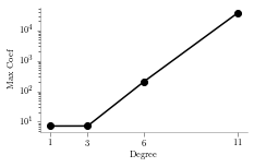

def cost(theta_0, theta_1, x, y):
    s = 0
    for i in range(len(x)):
        y_i_hat = x[i]*theta_1 + theta_0
        s += (y[i]-y_i_hat)**2
    return s/len(x)

x_grid, y_grid = np.mgrid[-4:15:.2, -4:15:.2]

cost_matrix = np.zeros_like(x_grid)
for i in range(x_grid.shape[0]):
    for j in range(x_grid.shape[1]):
        cost_matrix[i, j] = cost(x_grid[i, j], y_grid[i, j], data['x'], data['y'])

from matplotlib.patches import Circle

levels = np.sort(np.array([2,10,20,50,100,150,200,400,600,800,1000]))

plt.contourf(x_grid, y_grid, cost_matrix, levels,alpha=.4)
plt.colorbar()
plt.axhline(0, color='black', alpha=.5, dashes=[2, 4],linewidth=1)
plt.axvline(0, color='black', alpha=0.5, dashes=[2, 4],linewidth=1)

CS = plt.contour(x_grid, y_grid, cost_matrix, levels, linewidths=1,colors='black')
plt.clabel(CS, inline=1, fontsize=8)
plt.title("Least squares objective function")
plt.xlabel(r"$\theta_0$")
plt.ylabel(r"$\theta_1$")
p1 = Circle((0, 0), 3, color='g', label=r'$\theta_0^2+\theta_1^2=3$')
plt.scatter([7], [4],marker='*', color='r',s=25,label='Actual Solution')
plt.gca().add_patch(p1)
plt.legend()
plt.gca().set_aspect('equal')
format_axes(plt.gca())
plt.savefig('ridge_base_contour.pdf', transparent=True, bbox_inches="tight")
plt.show()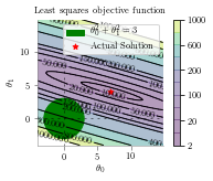

fig = plt.figure(figsize=(7,7))
ax = plt.axes(projection='3d')

ax = plt.axes(projection='3d')
ax.plot_surface(x_grid, y_grid, cost_matrix,cmap='viridis', edgecolor='none')
ax.set_title('Least squares objective function');
ax.set_xlabel(r"$\theta_0$")
ax.set_ylabel(r"$\theta_1$")
ax.set_xlim([-4,15])
ax.set_ylim([-4,15])

u = np.linspace(0, np.pi, 30)
v = np.linspace(0, 2 * np.pi, 30)

# x = np.outer(500*np.sin(u), np.sin(v))
# y = np.outer(500*np.sin(u), np.cos(v))
# z = np.outer(500*np.cos(u), np.ones_like(v))
# ax.plot_wireframe(x, y, z)

ax.view_init(45, 120)
plt.savefig('ridge_base_surface.pdf', transparent=True, bbox_inches="tight")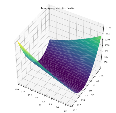

latexify(fig_width=5, fig_height=2.5)
from sklearn.linear_model import Ridge

for alpha in [1, 10, 1000]:
    fig, ax = plt.subplots(nrows=1, ncols=2)
    
    deg = 1
    predictors = ['ones','x']
    if deg >= 2:
        predictors.extend(['x_%d'%i for i in range(2,deg+1)])  

    regressor = Ridge(alpha=alpha,normalize=True, fit_intercept=False)
    regressor.fit(data[predictors],data['y'])
    y_pred = regressor.predict(data[predictors])
    format_axes(ax[0])
    format_axes(ax[1])
    # Plot
    ax[0].scatter(data['x'],data['y'], label='Train')
    ax[0].plot(data['x'], y_pred,'k', label='Prediction')
    ax[0].plot(data['x'], y_true,'g.', label='True Function')
    ax[0].legend() 
    ax[0].set_title(f"Degree: {deg} | $\mu$: {alpha} | Max Coef: {max(regressor.coef_, key=abs):.2f}")

    # Circle
    p1 = Circle((0, 0), np.sqrt(regressor.coef_.T@regressor.coef_), alpha=0.6, color='g', label=r'$\theta_0^2+\theta_1^2={:.2f}$'.format(np.sqrt(regressor.coef_.T@regressor.coef_)))
    ax[1].add_patch(p1)

    # Contour
    levels = np.sort(np.array([2,10,20,50,100,150,200,400,600,800,1000]))
    ax[1].contourf(x_grid, y_grid, cost_matrix, levels,alpha=.3)
    #ax[1].colorbar()
    ax[1].axhline(0, color='black', alpha=.5, dashes=[2, 4],linewidth=1)
    ax[1].axvline(0, color='black', alpha=0.5, dashes=[2, 4],linewidth=1)

    CS = plt.contour(x_grid, y_grid, cost_matrix, levels, linewidths=1,colors='black')
    ax[1].clabel(CS, inline=1, fontsize=8)
    ax[1].set_title("Least squares objective function")
    ax[1].set_xlabel(r"$\theta_0$")
    ax[1].set_ylabel(r"$\theta_1$")
    ax[1].scatter(regressor.coef_[0],regressor.coef_[1] ,marker='x', color='r',s=25,label='Ridge Solution')
    ax[1].scatter([7], [4],marker='*', color='r',s=25,label='Actual Solution')
    ax[1].set_xlim([-4,15])
    ax[1].set_ylim([-4,15])
    ax[1].legend()
    ax[1].set_aspect('equal')
    plt.savefig('ridge_{}.pdf'.format(alpha), transparent=True, bbox_inches="tight")
    plt.show()
    plt.clf()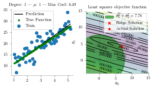

<Figure size 360x180 with 0 Axes>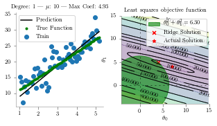

<Figure size 360x180 with 0 Axes>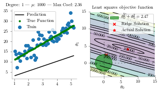

<Figure size 360x180 with 0 Axes>

latexify()
from sklearn.linear_model import Ridge

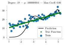
for i,deg in enumerate([19]):
    predictors = ['ones', 'x']
    if deg >= 2:
        predictors.extend(['x_%d'%i for i in range(2,deg+1)])  

    for i,alpha in enumerate([1, 1e7]):
        regressor = Ridge(alpha=alpha,normalize=False, fit_intercept=False)
        regressor.fit(data[predictors],data['y'])
        y_pred = regressor.predict(data[predictors])
        plt.scatter(data['x'],data['y'], label='Train')
        plt.plot(data['x'], y_pred,'k', label='Prediction')
        plt.plot(data['x'], y_true,'g.', label='True Function')
        plt.legend() 
        format_axes(plt.gca())
        plt.title(f"Degree: {deg} | $\mu$: {alpha} | Max Coeff: {max(regressor.coef_, key=abs):.2f}")
        plt.savefig('ridge_{}_{}.pdf'.format(alpha, deg), transparent=True, bbox_inches="tight")
        plt.show()
        plt.clf()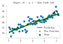

<Figure size 244.08x150.85 with 0 Axes>

# from sklearn.linear_model import Ridge

# for i,deg in enumerate([2,4,8,16]):
#   predictors = ['x']
#   if deg >= 2:
#     predictors.extend(['x_%d'%i for i in range(2,deg+1)])  
#   fig, ax = plt.subplots(nrows=1, ncols=4, sharey=True, figsize=(20, 4))

#   for i,alpha in enumerate([1e-15,1e-4,1,20]):
#     regressor = Ridge(alpha=alpha,normalize=True)
#     regressor.fit(data[predictors],data['y'])
#     y_pred = regressor.predict(data[predictors])
#     ax[i].scatter(data['x'],data['y'], label='Train')
#     ax[i].plot(data['x'], y_pred,'k', label='Prediction')
#     ax[i].plot(data['x'], y_true,'g.', label='True Function')
#     ax[i].legend() 
#     ax[i].set_title(f"Degree: {deg} | Alpha: {alpha} | Max Coeff: {max(regressor.coef_, key=abs):.2f}")

import pandas as pd

data = pd.read_excel("data.xlsx")
cols = data.columns
alph_list = np.logspace(-2,10,num=20, endpoint=False)
coef_list = []

for i,alpha in enumerate(alph_list):
    regressor = Ridge(alpha=alpha,normalize=True)
    regressor.fit(data[cols[1:-1]],data[cols[-1]])
    coef_list.append(regressor.coef_)

coef_list = np.abs(np.array(coef_list).T)
for i in range(len(cols[1:-1])):
    plt.loglog(alph_list, coef_list[i] , label=r"$\theta_{}$".format(i))
plt.xlabel('$\mu$ value')
plt.ylabel('Coefficient Value')
plt.legend() 
format_axes(plt.gca())

lim = True
if lim:
    plt.ylim((10e-20, 100))
    plt.savefig('rid_reg-without-lim.pdf', transparent=True, bbox_inches="tight")
else:
    plt.savefig('rid_reg-with-lim.pdf', transparent=True, bbox_inches="tight")

# plt.set_title(f"Degree: {deg} | Alpha: {alpha} | Max Coeff: {max(regressor.coef_, key=abs):.2f}")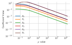

Question

plt.style.use('seaborn-whitegrid')

x = [1,2,3,4]
y = [1,2,3,0]
y_1 = [(2-i/5) for i in x]
y_2 = [(0.5+0.4*i) for i in x]
plt.ylim(-0.2,3.3)
plt.plot(x,y,'.')
for i in range(len(x)):
    plt.text(x[i]-0.1, y[i]+0.1, "({},{})".format(x[i], y[i]))
#plt.plot(x,y_1, label="unreg")
#plt.plot(x,y_2, label="reg")
#plt.legend()
#format_axes(plt.gca())
plt.savefig('temp.pdf', transparent=True)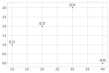

from sklearn.linear_model import LinearRegression
x_new = np.vstack([np.ones_like(x), x]).T
regressor = LinearRegression(normalize=False, fit_intercept=False)  
regressor.fit(x_new,y)
y_pred = regressor.predict(x_new)

for i in range(len(x)):
    plt.text(x[i]-0.1, y[i]+0.1, "({},{})".format(x[i], y[i]))
plt.plot(x,y,'.', label='Data Points')
plt.plot(x,y_pred,'-g', label='Unregularized Fit')
plt.legend(loc='lower left')
#format_axes(plt.gca())
plt.savefig('q_unreg.pdf', transparent=True)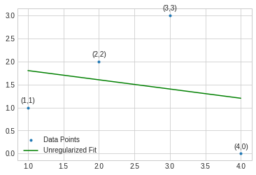

from sklearn.linear_model import Ridge

regressor = Ridge(alpha=4, normalize=False, fit_intercept=False)  
regressor.fit(x_new,y)
y_pred_r = regressor.predict(x_new)

for i in range(len(x)):
    plt.text(x[i]-0.1, y[i]+0.1, "({},{})".format(x[i], y[i]))
def ridge_func(x):
    return 0.56 + 0.26*np.array(x)
plt.plot(x,y,'.', label='Data Points')
plt.plot(x,y_pred,'-g', label='Unregularized Fit')
plt.plot(x,ridge_func(x),'-b', label='Regularized Fit')
plt.legend(loc='lower left')
#format_axes(plt.gca())
plt.savefig('q_reg.pdf', transparent=True)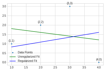

regressor.coef_

array([0.37209302, 0.30232558])

Retrying with a better example

np.linalg.inv([[4, 10], [10, 34]])@np.array([6, 14])

array([ 1.77777778, -0.11111111])

np.linalg.inv([[8, 10], [10, 34]])@np.array([6, 14])

array([0.37209302, 0.30232558])

#Define input array with angles from 60deg to 300deg converted to radians
x = np.array([i*np.pi/180 for i in range(60,600,10)])
np.random.seed(10)  #Setting seed for reproducability
y = 4*x + 7 + np.random.normal(0,5,len(x))
y_true = 4*x + 7
max_deg = 20
data_x = [x**(i+1) for i in range(max_deg)] + [y]
data_c = ['x'] + ['x_{}'.format(i+1) for i in range(1,max_deg)] + ['y']
data = pd.DataFrame(np.column_stack(data_x),columns=data_c)
data["ones"] = 1
plt.plot(data['x'],data['y'],'.', label='Data Points')
plt.plot(data['x'], y_true,'g', label='True Function')
plt.xlabel("x")
plt.ylabel("y")
plt.legend()
#format_axes(plt.gca())
plt.savefig('lin_1.pdf', transparent=True, bbox_inches="tight")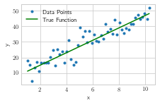

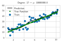
from sklearn.linear_model import Ridge

for i,deg in enumerate([17]):
    predictors = ['ones', 'x']
    if deg >= 2:
        predictors.extend(['x_%d'%i for i in range(2,deg+1)])  

    for i,alpha in enumerate([1e-3, 1e7]):
        regressor = Ridge(alpha=alpha,normalize=False)
        regressor.fit(data[predictors],data['y'])
        y_pred = regressor.predict(data[predictors])
        plt.scatter(data['x'],data['y'], label='Train')
        plt.plot(data['x'], y_pred,'k', label='Prediction')
        plt.plot(data['x'], y_true,'g.', label='True Function')
        plt.legend() 
        #format_axes(plt.gca())
        #print(regressor.coef_)
        plt.ylim([0,60])
        plt.title(f"Degree: {deg} | $\mu$: {alpha}")
        plt.savefig('ridge_new_{}_{}.pdf'.format(i, deg), transparent=True, bbox_inches="tight")
        plt.show()
        plt.clf()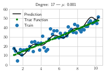

<Figure size 244.08x150.85 with 0 Axes>