Hierarchical Clustering

Hierarchical Clustering

import numpy as np
import matplotlib.pyplot as plt
import pandas as pd

%matplotlib inline
%config InlineBackend.figure_format = 'retina'

from sklearn.datasets import make_blobs
from sklearn.cluster import KMeans

# Create a dataset with K_dataset clusters
K_dataset = 3

X, y = make_blobs(n_samples=10, centers=K_dataset, n_features=2, random_state=0)

plt.scatter(X[:, 0], X[:, 1], c=y, s=200, cmap='viridis')
# Annotate sample number
for i in range(X.shape[0]):
    plt.annotate(i, (X[i, 0], X[i, 1]), fontsize=20)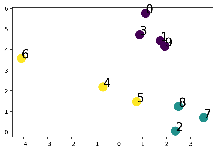

# Show after 1 step of hierarchical clustering
from scipy.cluster.hierarchy import dendrogram, linkage

Z = linkage(X, 'average')
plt.figure(figsize=(10, 5))

dendrogram(Z, labels=range(X.shape[0]), leaf_rotation=90, leaf_font_size=20)
plt.show()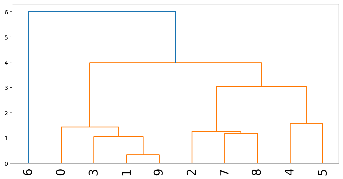

# Pairwise distance matrix
from scipy.spatial.distance import pdist, squareform

# Compute the distance matrix
dist = pdist(X, metric='euclidean')
dist = squareform(dist)
X_index = [f"P{x}" for x in np.arange(X.shape[0])]
df = pd.DataFrame(dist, index=X_index, columns=X_index)
df

	P0	P1	P2	P3	P4	P5	P6	P7	P8	P9
P0	0.000000	1.468503	5.849187	1.072565	4.001437	4.311101	5.641206	5.617833	4.732056	1.796596
P1	1.468503	0.000000	4.427098	0.911272	3.289419	3.124431	5.879548	4.149512	3.283718	0.332095
P2	5.849187	4.427098	0.000000	4.904326	3.705648	2.158345	7.350236	1.347556	1.194950	4.132565
P3	1.072565	0.911272	4.904326	0.000000	2.966927	3.253476	5.083095	4.830950	3.843925	1.193839
P4	4.001437	3.289419	3.705648	2.966927	0.000000	1.575484	3.691478	4.465344	3.299630	3.257210
P5	4.311101	3.124431	2.158345	3.253476	1.575484	0.000000	5.263313	2.910477	1.771561	2.937847
P6	5.641206	5.879548	7.350236	5.083095	3.691478	5.263313	0.000000	8.154381	6.982831	6.034281
P7	5.617833	4.149512	1.347556	4.830950	4.465344	2.910477	8.154381	0.000000	1.180379	3.821671
P8	4.732056	3.283718	1.194950	3.843925	3.299630	1.771561	6.982831	1.180379	0.000000	2.976718
P9	1.796596	0.332095	4.132565	1.193839	3.257210	2.937847	6.034281	3.821671	2.976718	0.000000

import seaborn as sns
# use lower triangle of matrix
mask = np.zeros_like(dist, dtype=np.bool_)
mask[np.triu_indices_from(mask)] = True
plt.figure(figsize=(10, 10))
# Make heatmap with seaborn and mask, mentining column and row names
sns.heatmap(dist, mask=mask, xticklabels=X_index, yticklabels=X_index, annot=True, cmap='viridis')

<AxesSubplot:>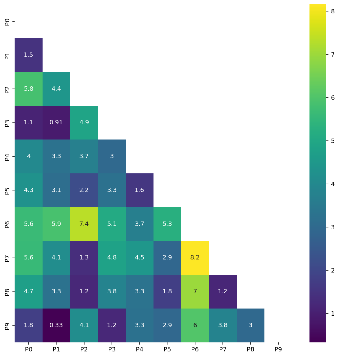

# Combine closest clusters 
# (i.e. the two clusters with the smallest distance)

# Find the two clusters with the smallest distance ignoring the diagonal
# (i.e. the distance between a cluster and itself)
np.fill_diagonal(dist, np.inf)
i, j= np.unravel_index(np.argmin(dist), dist.shape)
print(i, j)

1 9

# Combine the two clusters to a single "point"
X_new = np.vstack([X[i], X[j]])
new_point_name = f'{i} & {j}'
new_point_value = X_new.mean(axis=0)
print(new_point_name, new_point_value)

# Add new point to the dataset, remove the two old points
X = np.vstack([X, new_point_value])
X = np.delete(X, [i, j], axis=0)
print(X.shape)
#Update X_index to reflect the new point and the removed points
X_index = [f"P{x}" for x in range(10) if x not in [i, j]]
X_index.append(new_point_name)

# Compute the distance matrix
dist = pdist(X, metric='euclidean')
dist = squareform(dist)
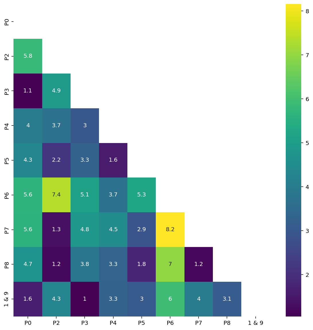
df = pd.DataFrame(dist, index=X_index, columns=X_index)

1 & 9 [1.83183315 4.28894623]
(9, 2)

df

	P0	P2	P3	P4	P5	P6	P7	P8	1 & 9
P0	0.000000	5.849187	1.072565	4.001437	4.311101	5.641206	5.617833	4.732056	1.632347
P2	5.849187	0.000000	4.904326	3.705648	2.158345	7.350236	1.347556	1.194950	4.279144
P3	1.072565	4.904326	0.000000	2.966927	3.253476	5.083095	4.830950	3.843925	1.048934
P4	4.001437	3.705648	2.966927	0.000000	1.575484	3.691478	4.465344	3.299630	3.269140
P5	4.311101	2.158345	3.253476	1.575484	0.000000	5.263313	2.910477	1.771561	3.028025
P6	5.641206	7.350236	5.083095	3.691478	5.263313	0.000000	8.154381	6.982831	5.955102
P7	5.617833	1.347556	4.830950	4.465344	2.910477	8.154381	0.000000	1.180379	3.985504
P8	4.732056	1.194950	3.843925	3.299630	1.771561	6.982831	1.180379	0.000000	3.129577
1 & 9	1.632347	4.279144	1.048934	3.269140	3.028025	5.955102	3.985504	3.129577	0.000000

mask = np.zeros_like(dist, dtype=np.bool_)
mask[np.triu_indices_from(mask)] = True
plt.figure(figsize=(10, 10))
# Make heatmap with seaborn and mask, mentining column and row names
sns.heatmap(dist, mask=mask, xticklabels=X_index, yticklabels=X_index, annot=True, cmap='viridis')

<AxesSubplot:>