# Create two 3d plot any theta_0, theta_1, theta_2
# First showing the decision boundary
# Second showing the probability of class 1
from mpl_toolkits.mplot3d import Axes3D
def plot_decision_boundary_3d(theta_0, theta_1, theta_2, azim=30, elev=30):
fig = plt.figure(figsize=(10, 8))
ax1 = fig.add_subplot(121, projection='3d')
ax2 = fig.add_subplot(122, projection='3d')
x_lin = np.linspace(-4, 4, 100)
y_lin = np.linspace(-4, 4, 100)
X_g, Y_g = np.meshgrid(x_lin, y_lin)
Z_g = -(theta_0 + theta_1 * X_g + theta_2 * Y_g)
#ax.plot_surface(X_g, Y_g, Z_g, alpha=0.2)
ax1.set_xlabel(r'$x_1$')
ax1.set_ylabel(r'$x_2$')
ax1.set_zlabel(r'$x_3$')
ax1.set_title(r'$\theta_0 = {:.2f}, \theta_1 = {:.2f}, \theta_2 = {:.2f}$'.format(theta_0, theta_1, theta_2))
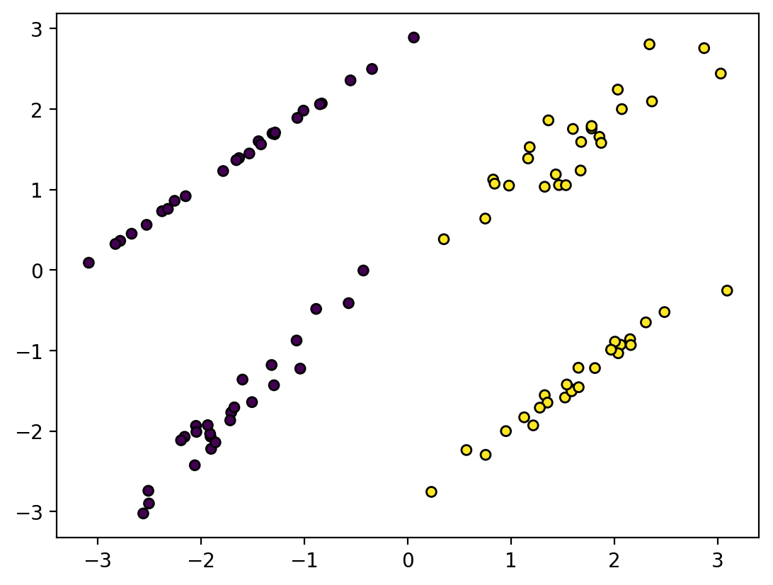
# Scatter plot of data (class 1 is Z = 1, class 0 is Z = 0)
ax1.scatter(X[y == 1, 0], X[y == 1, 1], 1, marker='o', c='b', s=25, edgecolor='k')
ax1.scatter(X[y == 0, 0], X[y == 0, 1], 0, marker='o', c='y', s=25, edgecolor='k')
# Plot the 3d sigmoid function
x1, x2 = np.meshgrid(np.linspace(-4, 4, 100), np.linspace(-4, 4, 100))
z = 1 / (1 + np.exp(-(theta_0 + theta_1 * x1 + theta_2 * x2)))
# Plot the decision plane
ax1.plot_surface(X_g, Y_g, Z_g, alpha=0.2, color='k')
# Plot the probability of class 1
ax2.plot_surface(x1, x2, z, alpha=0.2, color='black')
ax2.scatter(X[y == 1, 0], X[y == 1, 1], 1, marker='o', c='b', s=25, edgecolor='k')
ax2.scatter(X[y == 0, 0], X[y == 0, 1], 0, marker='o', c='y', s=25, edgecolor='k')
# Rotate the plot so that the sigmoid function is visible
ax1.view_init(azim, elev)
ax2.view_init(azim, elev)