import torch
import numpy as np
import pandas as pd
import matplotlib.pyplot as plt
%matplotlib inline
# Retina display
%config InlineBackend.figure_format = 'retina'

from tueplots import bundles
plt.rcParams.update(bundles.beamer_moml())

# Also add despine to the bundle using rcParams
plt.rcParams['axes.spines.right'] = False
plt.rcParams['axes.spines.top'] = False

# Increase font size to match Beamer template
plt.rcParams['font.size'] = 16
# Make background transparent
plt.rcParams['figure.facecolor'] = 'none'

import logging
logging.getLogger('matplotlib.font_manager').disabled = True

from ipywidgets import interact, FloatSlider, IntSliderSetting Up & Imports
Coin Toss Problem
def plot_beta(alpha, beta):
    dist = torch.distributions.Beta(concentration1=alpha, concentration0=beta)
    xs = torch.linspace(0, 1, 500)
    ys = dist.log_prob(xs).exp()
    plt.plot(xs, ys, color="C0")
    plt.grid()
    plt.xlabel(r"$\theta$")
    plt.ylabel(r"$p(\theta)$")
    plt.title("Beta Distribution")
    plt.show()


interact(
    plot_beta,
    alpha=FloatSlider(min=1, max=11, step=0.5, value=1),
    beta=FloatSlider(min=1, max=11, step=0.5, value=1),
)
<function __main__.plot_beta(alpha, beta)>combinations = [[1, 1], [5, 1], [1, 3], [2, 2], [2, 5]]
fig, ax = plt.subplots(1, 1)
for alpha, beta in combinations:
dist = torch.distributions.Beta(concentration1=alpha, concentration0=beta)
xs = torch.linspace(0, 1, 500)
ys = dist.log_prob(xs).exp()
ax.plot(xs, ys, label=rf"($\alpha$={alpha}, $\beta$={beta})")
ax.legend()
ax.grid()
ax.set_xlabel(r"$\theta$")
ax.set_ylabel(r"$p(\theta)$")
ax.set_title("Beta Distribution")
ax.set_ylim(0, 3)
plt.savefig("../figures/map/beta_distribution.pdf", bbox_inches="tight")
plt.show()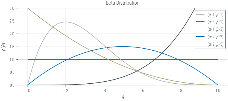
alpha = 11
beta = 11
bernoulli_theta = 0.5
n_1 = 9
n_0 = 1

dist = torch.distributions.Beta(concentration1=alpha, concentration0=beta)
xs = torch.linspace(0, 1, 500)
ys = dist.log_prob(xs).exp()
plt.plot(xs, ys, label="Beta Prior")

sample_size = n_1 + n_0
plt.title(f"H: {n_1}, T: {n_0}")

mle_estimate = n_1 / (sample_size)  # samples.mean()
plt.axvline(mle_estimate, color="k", linestyle="--", label="MLE")

map_estimate = (n_1 + alpha - 1) / (sample_size + alpha + beta - 2)
plt.axvline(map_estimate, color="r", linestyle="-.", label="MAP")

plt.axvline(alpha / (alpha + beta), color="g", linestyle=":", label="Prior Mean")

plt.grid()
plt.xlabel(r"$\theta$")
plt.ylabel(r"$p(\theta)$")
plt.legend(bbox_to_anchor=(1.25, 1), borderaxespad=0)
plt.savefig("../figures/map/coin_toss_prior_mle_map.pdf", bbox_inches="tight")
plt.show()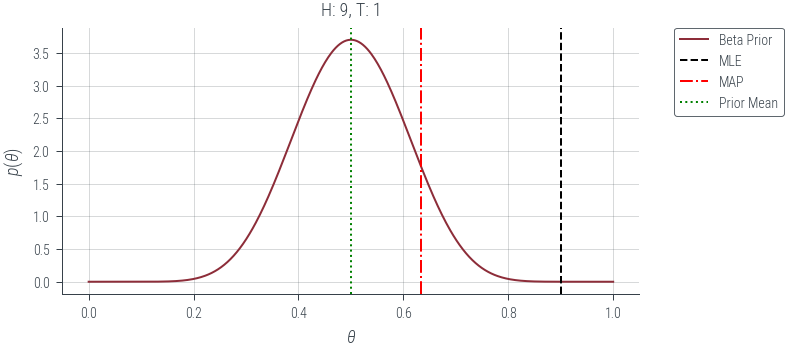
def plot_beta_all(alpha, beta, bernoulli_theta=0.5, sample_size=10):
    torch.manual_seed(42)

    dist = torch.distributions.Beta(concentration1=alpha, concentration0=beta)
    xs = torch.linspace(0, 1, 500)
    ys = dist.log_prob(xs).exp()
    plt.plot(xs, ys, label="Beta Prior")

    samples = torch.empty(sample_size)
    for s_num in range(sample_size):
        dist = torch.distributions.Bernoulli(probs=bernoulli_theta)
        samples[s_num] = dist.sample()
    n_1 = int(samples.sum())
    n_0 = int(sample_size - n_1)
    plt.title(f"H: {n_1}, T: {n_0}")

    mle_estimate = n_1 / (sample_size)  # samples.mean()
    plt.axvline(mle_estimate, color="k", linestyle="--", label="MLE")

    map_estimate = (n_1 + alpha - 1) / (sample_size + alpha + beta - 2)
    plt.axvline(map_estimate, color="r", linestyle="-.", label="MAP")

    plt.axvline(alpha / (alpha + beta), color="g", linestyle=":", label="Prior Mean")

    plt.grid()
    plt.xlabel(r"$\theta$")
    plt.ylabel(r"$p(\theta)$")
    plt.legend(bbox_to_anchor=(1.25, 1), borderaxespad=0)
    plt.show()


interact(
    plot_beta_all,
    alpha=FloatSlider(min=1, max=51, step=1, value=11),
    beta=FloatSlider(min=1, max=51, step=1, value=11),
    bernoulli_theta=FloatSlider(min=0, max=1, step=0.1, value=0.5),
    sample_size=IntSlider(min=10, max=1000, step=10, value=10),
)
<function __main__.plot_beta_all(alpha, beta, bernoulli_theta=0.5, sample_size=10)>Linear Regression
n_data = 20
x = torch.linspace(-1, 1, n_data)
slope = 2
intercept = 1
f = lambda x: slope * x + intercept

noise = torch.distributions.Normal(0, 1).sample((n_data,))
y = f(x) + noise

plt.figure()
plt.scatter(x, y, marker="x", c="k", s=20, label="Noisy data")
plt.plot(x, f(x), c="k", label="True function")
plt.xlabel("x")
plt.ylabel("y")
line_str = f"{slope} x + {intercept}"
plt.title(r"$y_{true} = $" + line_str)
plt.savefig(f"../figures/map/linreg_data-{n_data}.pdf", bbox_inches="tight")
plt.legend()
<matplotlib.legend.Legend at 0x7f2b9d6409d0>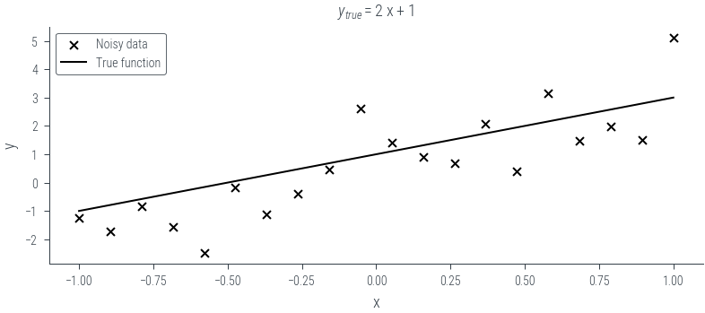
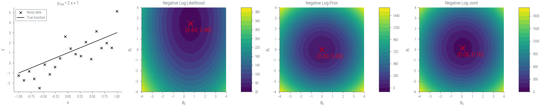
def nll(theta):
    mu = theta[0] + theta[1] * x
    sigma = torch.tensor(1.0)
    dist = torch.distributions.normal.Normal(mu, sigma)
    return -dist.log_prob(y).sum()


def neg_log_prior(theta):
    prior_mean = torch.tensor([0.0, 0.0])  # Prior mean for slope and intercept
    prior_std = torch.tensor(
        [0.1, 0.1]
    )  # Prior standard deviation for slope and intercept
    dist = torch.distributions.normal.Normal(prior_mean, prior_std)
    return -dist.log_prob(theta).sum()


def neg_log_joint(theta):
    return nll(theta) + neg_log_prior(theta)
# Create a grid of theta[0] and theta[1] values
theta0_values = torch.linspace(-4, 4, 101)
theta1_values = torch.linspace(-4, 4, 101)
theta0_mesh, theta1_mesh = torch.meshgrid(theta0_values, theta1_values)
nll_values = torch.zeros_like(theta0_mesh)
nlp_values = torch.zeros_like(theta0_mesh)
nlj_values = torch.zeros_like(theta0_mesh)
for i in range(len(theta0_values)):
for j in range(len(theta1_values)):
theta_current = torch.tensor([theta0_values[i], theta1_values[j]])
nll_values[i, j] = nll(theta_current)
nlp_values[i, j] = neg_log_prior(theta_current)
nlj_values[i, j] = neg_log_joint(theta_current)def plot_contour_with_minima(values, theta0_values, theta1_values, title, ax, cbar_ax):
# plt.figure(figsize=(6, 6))
contour = ax.contourf(theta0_mesh, theta1_mesh, values, levels=20, cmap="viridis")
ax.set_xlabel(r"$\theta_0$")
ax.set_ylabel(r"$\theta_1$")
ax.set_title(title)
ax.set_aspect("equal", adjustable="box") # Set aspect ratio to be equal
# mark the minimum
min_idx = np.unravel_index(np.argmin(values), values.shape)
t0_min = theta0_values[min_idx[0]]
t1_min = theta1_values[min_idx[1]]
ax.scatter(
t0_min,
t1_min,
marker="x",
color="red",
s=100,
)
ax.annotate(
f"({t0_min:.2f}, {t1_min:.2f})",
(t0_min, t1_min),
xytext=(t0_min - 0.5, t1_min - 0.8),
color="red",
# set size of text
size=12,
)
fig.colorbar(contour, ax=ax, cax=cbar_ax)
# plt.tight_layout()
# plt.show()
# return contour
# Usage example
fig, ax = plt.subplots(
1, 7, figsize=(15, 3), gridspec_kw={"width_ratios": [10, 10, 1, 10, 1, 10, 1]}
)
i = 0
def get_next_ax():
global i
i += 1
return ax[i - 1]
data_ax = get_next_ax()
data_ax.scatter(x, y, marker="x", c="k", s=20, label="Noisy data")
data_ax.plot(x, f(x), c="k", label="True function")
data_ax.set_xlabel("x")
data_ax.set_ylabel("y")
line_str = f"{slope} x + {intercept}"
data_ax.set_title(r"$y_{true} = $" + line_str)
data_ax.legend()
contour = plot_contour_with_minima(
nll_values,
theta0_values,
theta1_values,
"Negative Log-Likelihood",
get_next_ax(),
get_next_ax(),
)
contour = plot_contour_with_minima(
nlp_values,
theta0_values,
theta1_values,
"Negative Log-Prior",
get_next_ax(),
get_next_ax(),
)
contour = plot_contour_with_minima(
nlj_values,
theta0_values,
theta1_values,
"Negative Log-Joint",
get_next_ax(),
get_next_ax(),
)