Vanilla Linear Regression

import numpy as np
import matplotlib.pyplot as plt
import pandas as pd
%matplotlib inline
# Retina display
%config InlineBackend.figure_format = 'retina'
from jax import random

import warnings
warnings.filterwarnings('ignore')

plt.rcParams['figure.constrained_layout.use'] = True

import seaborn as sns
sns.set_context("notebook")

URL = "https://gist.githubusercontent.com/ucals/" + "2cf9d101992cb1b78c2cdd6e3bac6a4b/raw/"+ "43034c39052dcf97d4b894d2ec1bc3f90f3623d9/"+ "osic_pulmonary_fibrosis.csv"

train = pd.read_csv(URL)
train.head()

	Patient	Weeks	FVC	Percent	Age	Sex	SmokingStatus
0	ID00007637202177411956430	-4	2315	58.253649	79	Male	Ex-smoker
1	ID00007637202177411956430	5	2214	55.712129	79	Male	Ex-smoker
2	ID00007637202177411956430	7	2061	51.862104	79	Male	Ex-smoker
3	ID00007637202177411956430	9	2144	53.950679	79	Male	Ex-smoker
4	ID00007637202177411956430	11	2069	52.063412	79	Male	Ex-smoker

train.describe()

	Weeks	FVC	Percent	Age
count	1549.000000	1549.000000	1549.000000	1549.000000
mean	31.861846	2690.479019	77.672654	67.188509
std	23.247550	832.770959	19.823261	7.057395
min	-5.000000	827.000000	28.877577	49.000000
25%	12.000000	2109.000000	62.832700	63.000000
50%	28.000000	2641.000000	75.676937	68.000000
75%	47.000000	3171.000000	88.621065	72.000000
max	133.000000	6399.000000	153.145378	88.000000

# Number of unique patients
train['Patient'].nunique()

176

#Number of records per patient
train['Patient'].value_counts().reset_index()['Patient'].value_counts().sort_index().plot(kind='bar')
plt.xlabel("Number of weeks")
plt.ylabel("Number of Patients")

Text(0, 0.5, 'Number of Patients')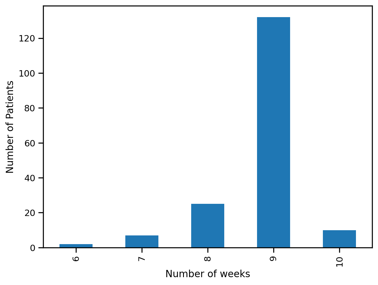

def chart_patient(patient_id, ax):
    data = train[train["Patient"] == patient_id]
    x = data["Weeks"]
    y = data["FVC"]
    ax.set_title(patient_id, fontsize=8)
    sns.regplot(x=x, y=y, ax=ax, ci=None, line_kws={"color": "black", "lw":2})


f, axes = plt.subplots(1, 3, sharey=True)
chart_patient("ID00007637202177411956430", axes[0])
chart_patient("ID00009637202177434476278", axes[1])
chart_patient("ID00010637202177584971671", axes[2])
f.tight_layout()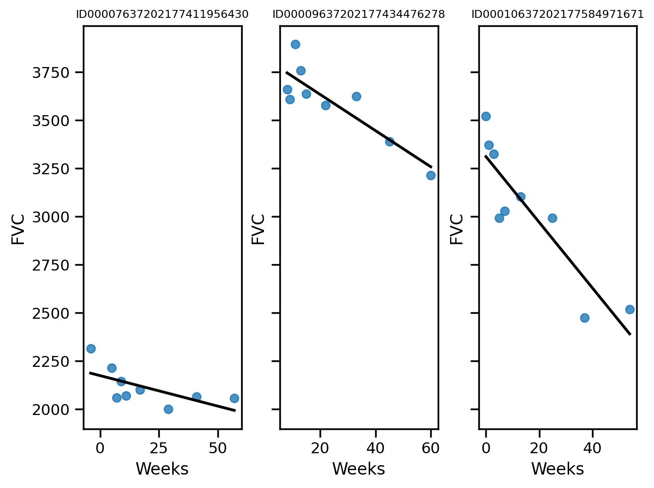

try:
    import numpyro
except ImportError:
    %pip install numpyro
    import numpyro

import numpyro.distributions as dist

sample_weeks = train["Weeks"].values
sample_fvc = train["FVC"].values

### Linear regression from scikit-learn
from sklearn.linear_model import LinearRegression

lr = LinearRegression()
lr.fit(sample_weeks.reshape(-1, 1), sample_fvc)

LinearRegression()

In a Jupyter environment, please rerun this cell to show the HTML representation or trust the notebook.
On GitHub, the HTML representation is unable to render, please try loading this page with nbviewer.org.

all_weeks = np.arange(-12, 134, 1)

# Plot the data and the regression line
plt.scatter(sample_weeks, sample_fvc, alpha=0.3)
plt.plot(all_weeks, lr.predict(all_weeks.reshape(-1, 1)), color="black", lw=2)
plt.xlabel("Weeks")
plt.ylabel("FVC")

Text(0, 0.5, 'FVC')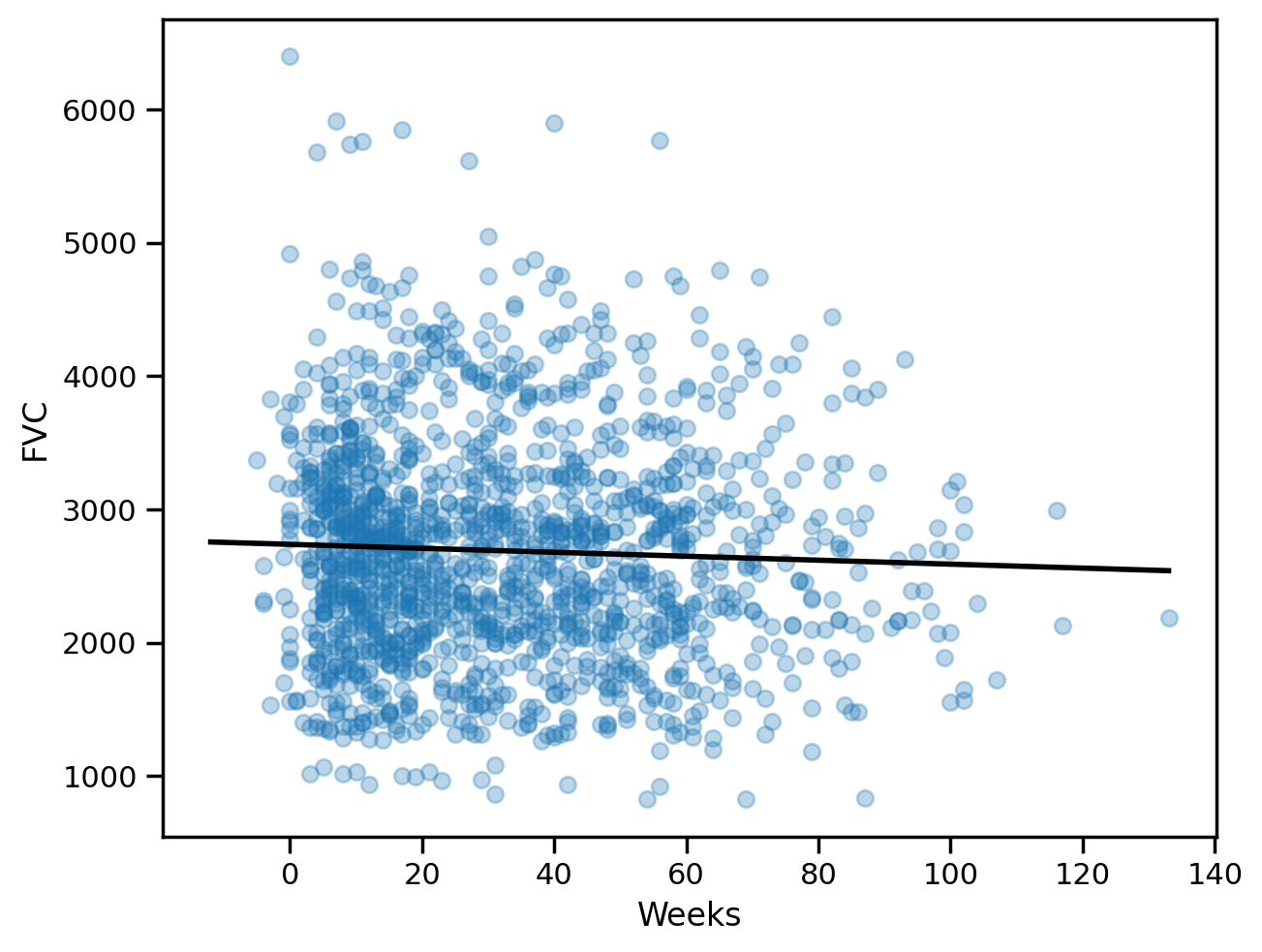

lr.coef_, lr.intercept_

(array([-1.48471319]), 2737.784722381955)

# Finding the mean absolute error

from sklearn.metrics import mean_absolute_error

maes = {}
maes["LinearRegression"] = mean_absolute_error(sample_fvc, lr.predict(sample_weeks.reshape(-1, 1)))
maes

{'LinearRegression': 654.8103093180237}

Pooled model

\(\alpha \sim \text{Normal}(0, 500)\)

\(\beta \sim \text{Normal}(0, 500)\)

\(\sigma \sim \text{HalfNormal}(100)\)

for i in range(N_Weeks):

\(FVC_i \sim \text{Normal}(\alpha + \beta \cdot Week_i, \sigma)\)

def pooled_model(sample_weeks, sample_fvc=None):
    α = numpyro.sample("α", dist.Normal(0., 500.))
    β = numpyro.sample("β", dist.Normal(0., 500.))
    σ = numpyro.sample("σ", dist.HalfNormal(50.))
    with numpyro.plate("samples", len(sample_weeks)):
        fvc = numpyro.sample("fvc", dist.Normal(α + β * sample_weeks, σ), obs=sample_fvc)
    return fvc

sample_weeks.shape

(1549,)

# Render the model graph
numpyro.render_model(pooled_model, model_kwargs={"sample_weeks": sample_weeks, "sample_fvc": sample_fvc},
                render_distributions=True,
                render_params=True,
                )

from sklearn.preprocessing import LabelEncoder

patient_encoder = LabelEncoder()
train["patient_code"] = patient_encoder.fit_transform(train["Patient"].values)

sample_patient_code = train["patient_code"].values

sample_patient_code

array([  0,   0,   0, ..., 175, 175, 175])

from numpyro.infer import MCMC, NUTS, Predictive

nuts_kernel = NUTS(pooled_model)

mcmc = MCMC(nuts_kernel, num_samples=4000, num_warmup=2000)
rng_key = random.PRNGKey(0)

WARNING:jax._src.xla_bridge:No GPU/TPU found, falling back to CPU. (Set TF_CPP_MIN_LOG_LEVEL=0 and rerun for more info.)

mcmc.run(rng_key, sample_weeks=sample_weeks, sample_fvc=sample_fvc)
posterior_samples = mcmc.get_samples()

sample: 100%|██████████| 6000/6000 [00:05<00:00, 1137.39it/s, 7 steps of size 5.24e-01. acc. prob=0.88]

import arviz as az

idata = az.from_numpyro(mcmc)
az.plot_trace(idata, compact=True);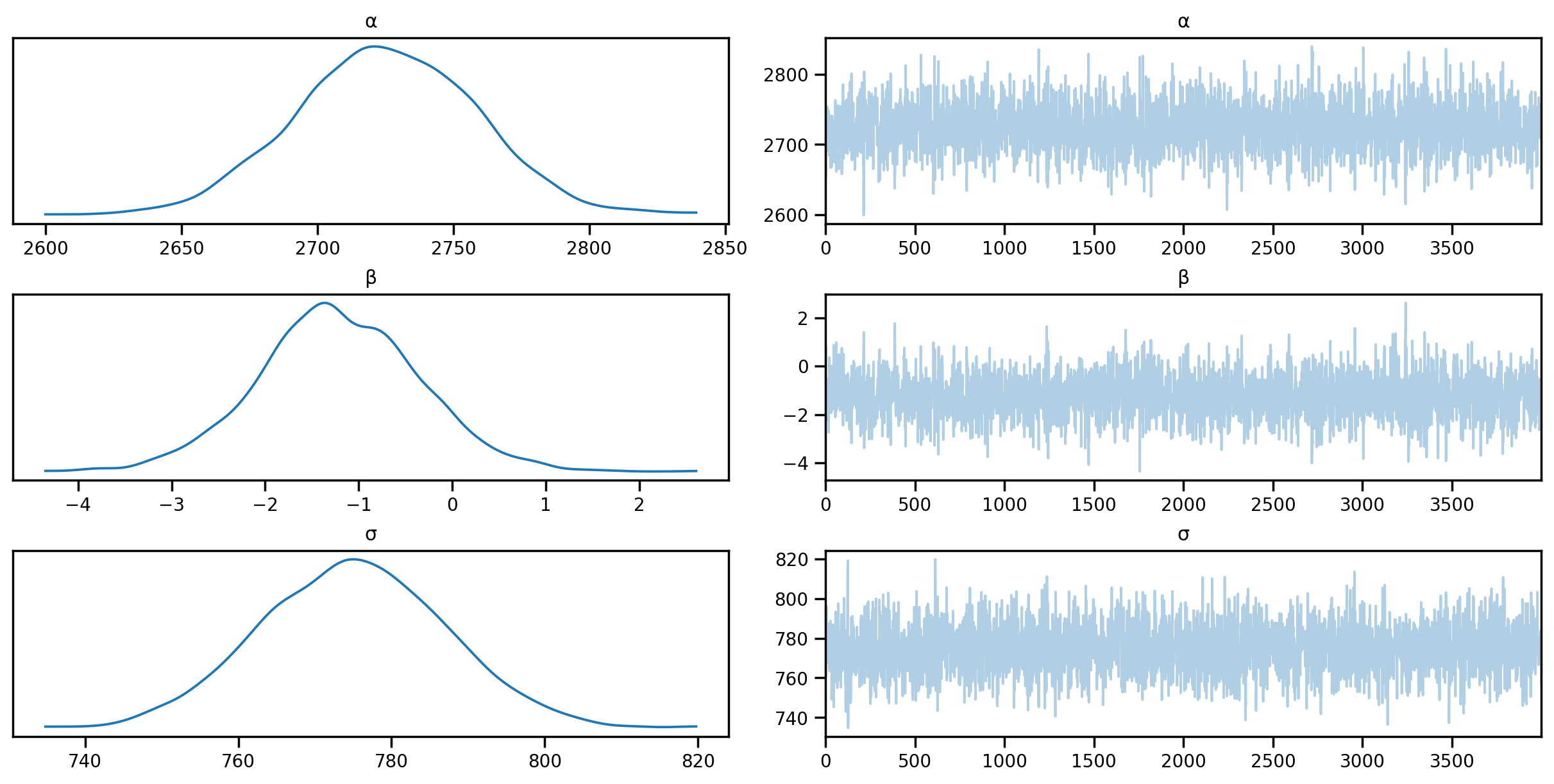

# Summary statistics
az.summary(idata, round_to=2)

Shape validation failed: input_shape: (1, 4000), minimum_shape: (chains=2, draws=4)

	mean	sd	hdi_3%	hdi_97%	mcse_mean	mcse_sd	ess_bulk	ess_tail	r_hat
α	2724.98	33.46	2663.52	2786.90	0.74	0.52	2052.67	1952.52	NaN
β	-1.22	0.85	-2.80	0.43	0.02	0.01	1955.95	2019.17	NaN
σ	775.05	12.03	752.85	797.95	0.25	0.17	2411.55	2720.36	NaN

# Predictive distribution
predictive = Predictive(pooled_model, mcmc.get_samples())

predictive

<numpyro.infer.util.Predictive at 0x7d2774b0b0a0>

predictions = predictive(rng_key, all_weeks, None)

pd.DataFrame(predictions["fvc"]).mean().plot()

<Axes: >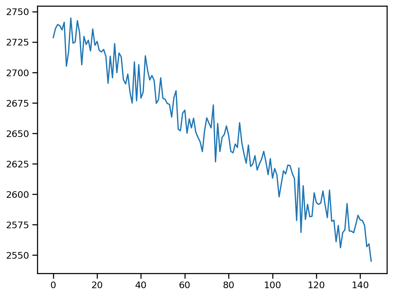

plt.plot(all_weeks, predictions["fvc"].mean(axis=0))
plt.scatter(sample_weeks, sample_fvc, alpha=0.1)

<matplotlib.collections.PathCollection at 0x7d2774851d50>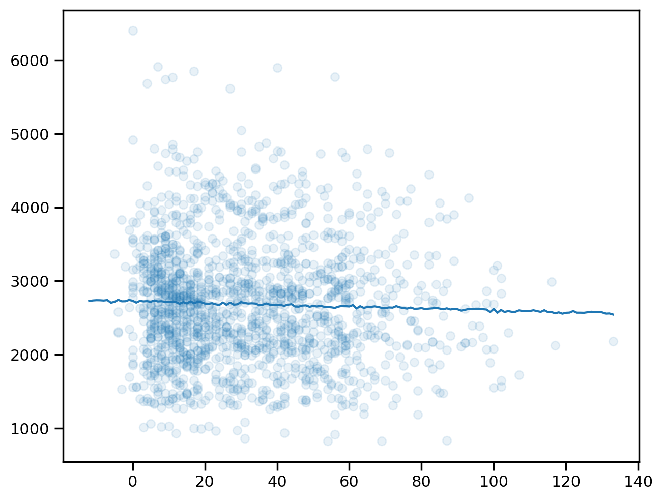

# Get the mean and standard deviation of the predictions
mu = predictions["fvc"].mean(axis=0)
sigma = predictions["fvc"].std(axis=0)

# Plot the predictions
plt.plot(all_weeks, mu)
plt.fill_between(all_weeks, mu - 1.96*sigma, mu + 1.96*sigma, alpha=0.2)
plt.scatter(sample_weeks, sample_fvc, alpha=0.2)
plt.xlabel("Weeks")
plt.ylabel("FVC")

Text(0, 0.5, 'FVC')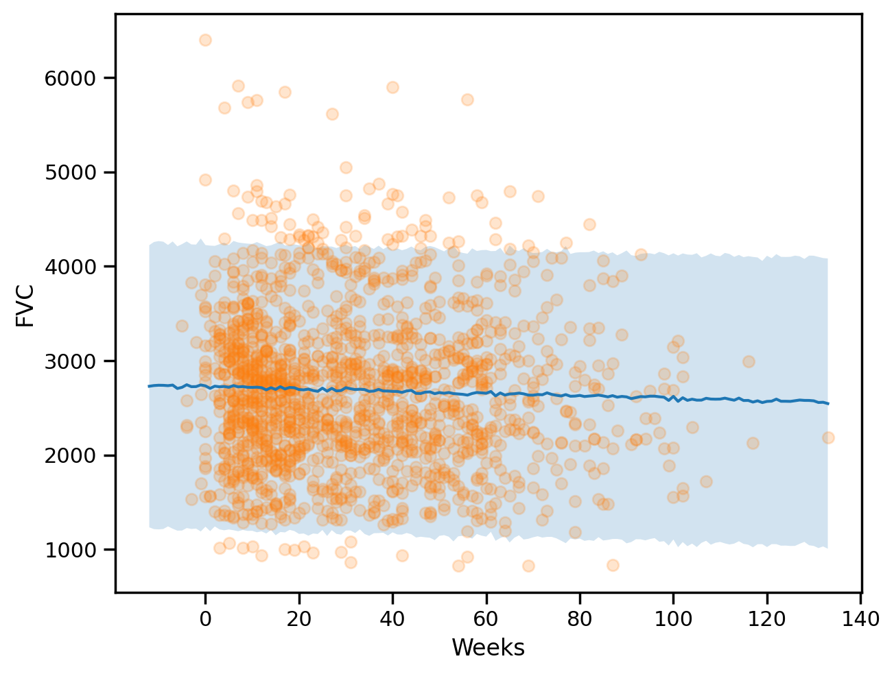

preds_pooled  = predictive(rng_key, sample_weeks, None)['fvc']
predictions_train_pooled = preds_pooled.mean(axis=0)
std_train_pooled = preds_pooled.std(axis=0)

### Computing Mean Absolute Error and Coverage at 95% confidence interval

maes["PooledModel"] = mean_absolute_error(sample_fvc, predictions_train_pooled)
maes

{'LinearRegression': 654.8103093180237, 'PooledModel': 654.6283571306085}

### Computing the coverage at 95% confidence interval

def coverage(y_true, y_pred, sigma):
    lower = y_pred - 1.96 * sigma
    upper = y_pred + 1.96 * sigma
    return np.mean((y_true >= lower) & (y_true <= upper))
coverages = {}
coverages["pooled"] = coverage(sample_fvc, predictions_train_pooled, std_train_pooled).item()
coverages

{'pooled': 0.9399612545967102}

The above numbers are comparable, which is a good sign. Let’s see if we can do better with a personalised model.

Unpooled Model

\(\sigma \sim \text{HalfNormal}(20)\)

---

for p in range(N_patients):

\(\alpha_p \sim \text{Normal}(0, 500)\)

\(\beta_p \sim \text{Normal}(0, 500)\)

---

for PAT in range(N_patients):
    for i in range(N_Weeks):

\(FVC_i \sim \text{Normal}(\alpha_{p}[PAT] + \beta_{p}[PAT] \cdot Week_i, \sigma)\)

# Unpooled model
def unpool_model(sample_weeks, sample_patient_code, sample_fvc=None):
    σ = numpyro.sample("σ", dist.HalfNormal(20.))
    with numpyro.plate("patients", sample_patient_code.max() + 1):
        α_p = numpyro.sample("α_p", dist.Normal(0, 500.))
        β_p = numpyro.sample("β_p", dist.Normal(0, 500.))
    with numpyro.plate("samples", len(sample_weeks)):
        fvc = numpyro.sample("fvc", numpyro.distributions.Normal(α_p[sample_patient_code] +
                                                                 β_p[sample_patient_code] * sample_weeks, σ),
                             obs=sample_fvc)
    return fvc

# Render the model graph

model_kwargs = {"sample_weeks": sample_weeks,
                "sample_patient_code": sample_patient_code,
                "sample_fvc": sample_fvc}

numpyro.render_model(unpool_model, model_kwargs=model_kwargs,
                render_distributions=True,
                render_params=True,
                )

nuts_kernel_unpooled = NUTS(unpool_model)

mcmc_unpooled = MCMC(nuts_kernel_unpooled, num_samples=200, num_warmup=500)
rng_key = random.PRNGKey(0)

model_kwargs

{'sample_weeks': array([-4,  5,  7, ..., 31, 43, 59]),
 'sample_patient_code': array([  0,   0,   0, ..., 175, 175, 175]),
 'sample_fvc': array([2315, 2214, 2061, ..., 2908, 2975, 2774])}

mcmc_unpooled.run(rng_key, **model_kwargs)

posterior_samples = mcmc_unpooled.get_samples()

sample: 100%|██████████| 700/700 [00:07<00:00, 90.53it/s, 63 steps of size 9.00e-02. acc. prob=0.91] 

az.plot_trace(az.from_numpyro(mcmc_unpooled), compact=True);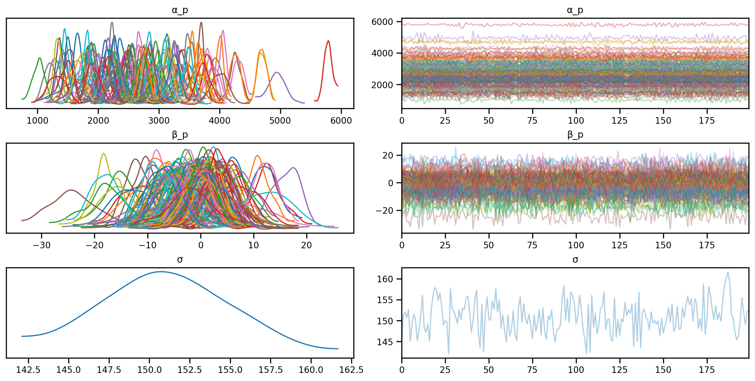

# Predictive distribution for unpooled model

predictive_unpooled = Predictive(unpool_model, mcmc_unpooled.get_samples())

# Predictive distribution for unpooled model for all weeks for a given patient

all_weeks = np.arange(-12, 134, 1)
def predict_unpooled(patient_code):
    predictions = predictive_unpooled(rng_key, all_weeks, patient_code)
    mu = predictions["fvc"].mean(axis=0)
    sigma = predictions["fvc"].std(axis=0)
    return mu, sigma

# Plot the predictions for a given patient
def plot_patient(patient_code):
    mu, sigma = predict_unpooled(patient_code)
    plt.plot(all_weeks, mu)
    plt.fill_between(all_weeks, mu - 1.96*sigma, mu + 1.96*sigma, alpha=0.6)
    id_to_patient = patient_encoder.inverse_transform(patient_code)[0]
    patient_weeks = train[train["Patient"] == id_to_patient]["Weeks"]
    patient_fvc = train[train["Patient"] == id_to_patient]["FVC"]
    plt.scatter(patient_weeks, patient_fvc, alpha=0.5)
    plt.xlabel("Weeks")
    plt.ylabel("FVC")
    plt.title(id_to_patient)

plot_pooled = False

def plot_total(patient_id = 0, plot_pooled = False):
  plot_patient(np.array([patient_id]))
  if plot_pooled:
      plt.plot(all_weeks, mu, color='g')
      plt.fill_between(all_weeks, mu - 1.96*sigma, mu + 1.96*sigma, alpha=0.05, color='g')

plot_total(0, True)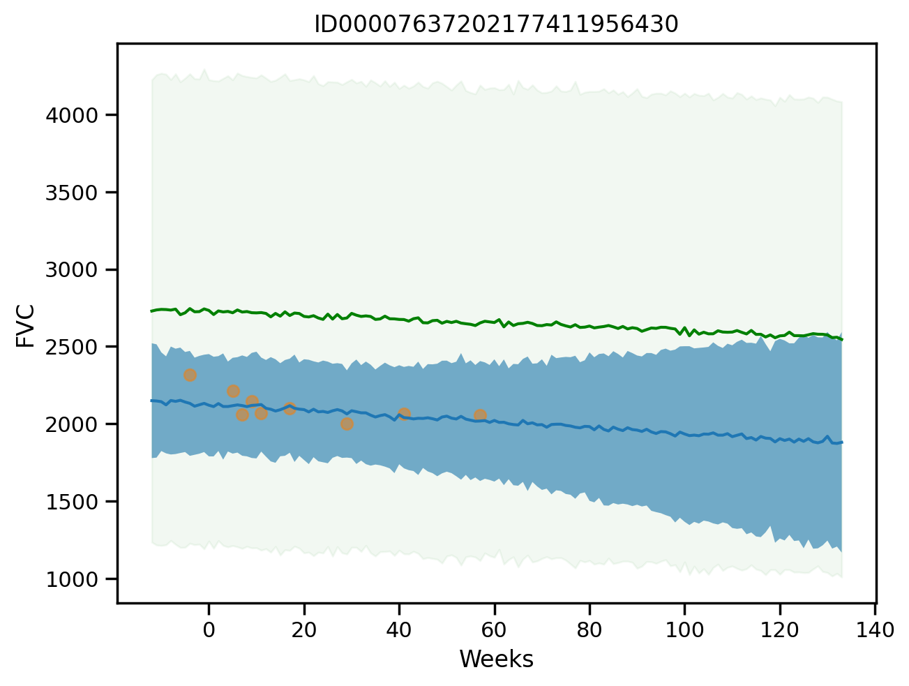

plot_total(0, True)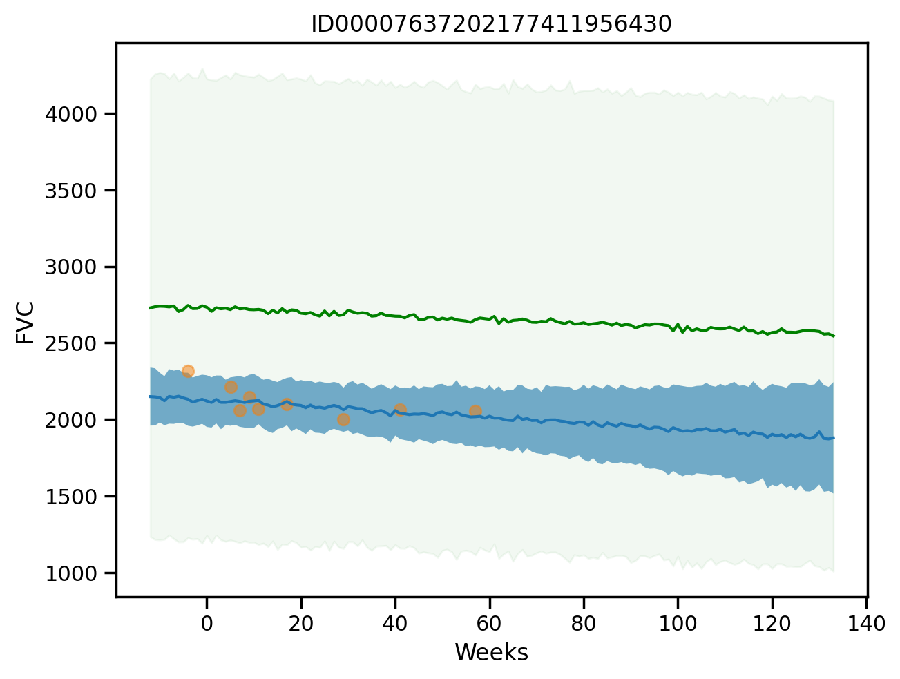

plot_total(1, True)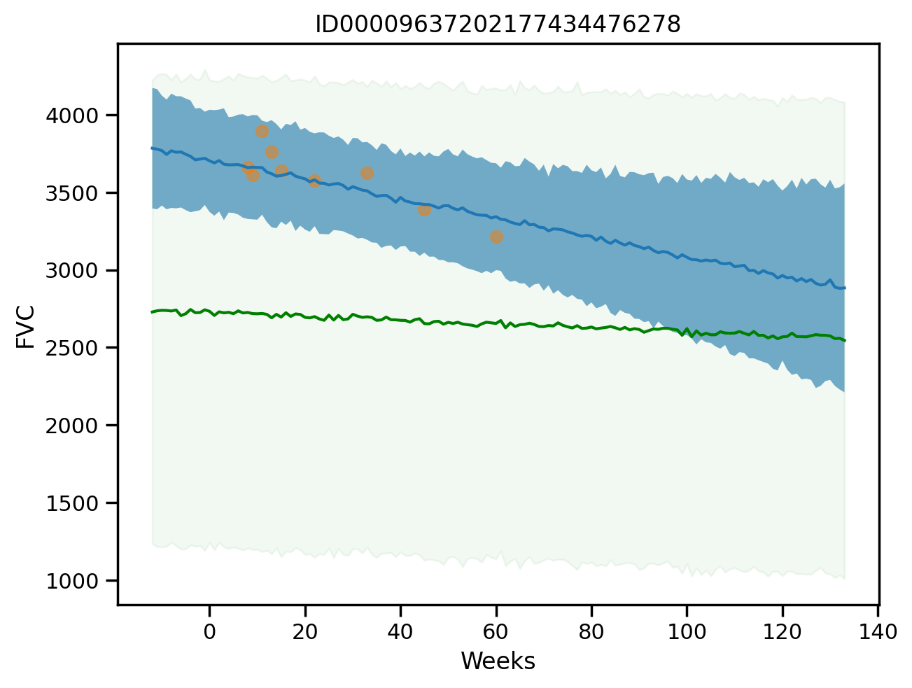

plot_total(3)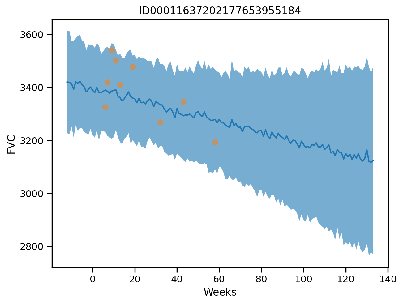

Computing metrics on the training set for unpool_model

predictions_train_unpooled = predictive_unpooled(rng_key,
                                                 sample_weeks,
                                                 train["patient_code"].values)['fvc']
predictions_train_unpooled.shape

(200, 1549)

mu_predictions_train_unpooled = predictions_train_unpooled.mean(axis=0)
std_predictions_train_unpooled = predictions_train_unpooled.std(axis=0)

maes["UnpooledModel"] = mean_absolute_error(sample_fvc, mu_predictions_train_unpooled)
maes

{'LinearRegression': 654.8103093180237,
 'PooledModel': 654.6283571306085,
 'UnpooledModel': 98.18583518632232}

coverages["unpooled"] = coverage(sample_fvc, mu_predictions_train_unpooled, std_predictions_train_unpooled).item()
coverages

{'pooled': 0.9399612545967102, 'unpooled': 0.974822461605072}

Exercise: Another variation of unpooled model

# Unpooled model
def unpool_model_var(sample_weeks, sample_patient_code, sample_fvc=None):
    with numpyro.plate("patients", sample_patient_code.max() + 1):
        α_p = numpyro.sample("α_p", dist.Normal(0, 500.))
        β_p = numpyro.sample("β_p", dist.Normal(0, 500.))
        σ_p = numpyro.sample("σ_p", dist.HalfNormal(20.))
    with numpyro.plate("samples", len(sample_weeks)):
        fvc = numpyro.sample("fvc", numpyro.distributions.Normal(α_p[sample_patient_code] +
                                                                 β_p[sample_patient_code] * sample_weeks,
                                                                 σ_p[sample_patient_code]),
                             obs=sample_fvc)
    return fvc

# Plot graphical model
numpyro.render_model(unpool_model_var, model_kwargs=model_kwargs,
                render_distributions=True,
                render_params=True,
                )

nuts_kernel_unpooled_2 = NUTS(unpool_model_var)

mcmc_unpooled_2 = MCMC(nuts_kernel_unpooled_2, num_samples=400, num_warmup=500)
rng_key = random.PRNGKey(0)

mcmc_unpooled_2.run(rng_key, **model_kwargs)

posterior_samples_2 = mcmc_unpooled_2.get_samples()

sample: 100%|██████████| 900/900 [00:08<00:00, 102.48it/s, 63 steps of size 8.17e-02. acc. prob=0.88]

az.plot_trace(az.from_numpyro(mcmc_unpooled_2), compact=True);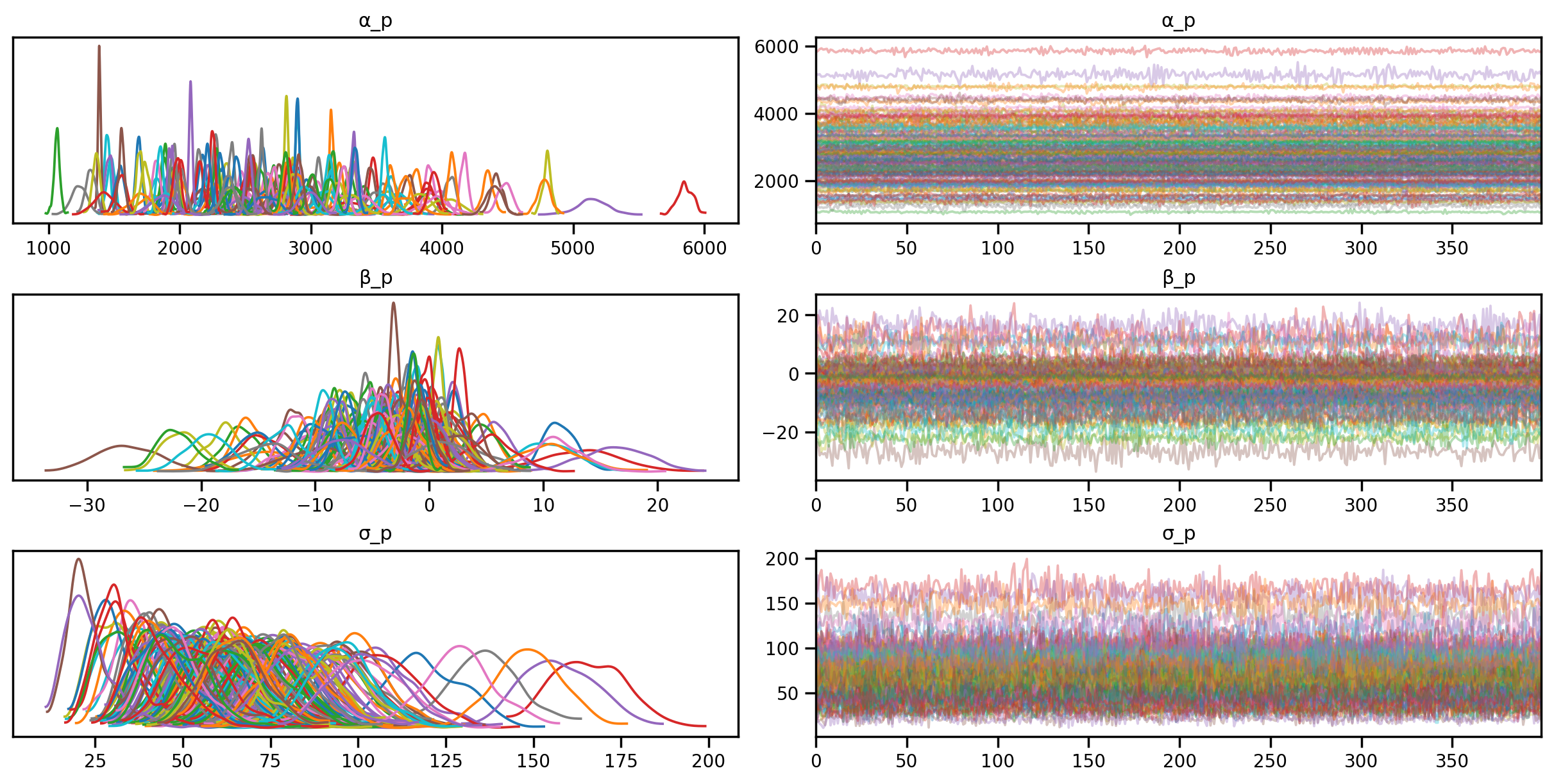

# Predictive distribution for unpooled model variation 2

predictive_unpooled_2 = Predictive(unpool_model_var, mcmc_unpooled_2.get_samples())

predictions_train_unpooled_2 = predictive_unpooled_2(rng_key,
                                                        sample_weeks,
                                                        train["patient_code"].values)['fvc']

mu_predictions_train_unpooled_2 = predictions_train_unpooled_2.mean(axis=0)
std_predictions_train_unpooled_2 = predictions_train_unpooled_2.std(axis=0)

maes["UnpooledModel2"] = mean_absolute_error(sample_fvc, mu_predictions_train_unpooled_2)

coverages["unpooled2"] = coverage(sample_fvc, mu_predictions_train_unpooled_2, std_predictions_train_unpooled_2).item()

print(maes)
print(coverages)

{'LinearRegression': 654.8103093180237, 'PooledModel': 654.6283571306085, 'UnpooledModel': 98.18583518632232, 'UnpooledModel2': 81.93005607511398}
{'pooled': 0.9399612545967102, 'unpooled': 0.974822461605072, 'unpooled2': 0.886378288269043}

Hierarchical model

\(\sigma \sim \text{HalfNormal}(100)\)

---

\(\mu_{\alpha} \sim \text{Normal}(0, 500)\)

\(\sigma_{\alpha} \sim \text{HalfNormal}(100)\)

\(\mu_{\beta} \sim \text{Normal}(0, 500)\)

\(\sigma_{\beta} \sim \text{HalfNormal}(100)\)

---

for p in range(N_patients):

\(\alpha_p \sim \text{Normal}(\mu_{\alpha}, \sigma_{\alpha})\)

\(\beta_p \sim \text{Normal}(\mu_{\beta}, \sigma_{\beta})\)

---

for i in range(N_Weeks):

\(FVC_i \sim \text{Normal}(\alpha_{p[i]} + \beta_{p[i]} \cdot Week_i, \sigma)\)

### Hierarchical model

def final_model(sample_weeks, sample_patient_code, sample_fvc=None):
    μ_α = numpyro.sample("μ_α", dist.Normal(0.0, 500.0))
    σ_α = numpyro.sample("σ_α", dist.HalfNormal(100.0))
    μ_β = numpyro.sample("μ_β", dist.Normal(0.0, 3.0))
    σ_β = numpyro.sample("σ_β", dist.HalfNormal(3.0))

    n_patients = len(np.unique(sample_patient_code))

    with numpyro.plate("Participants", n_patients):
        α = numpyro.sample("α", dist.Normal(μ_α, σ_α))
        β = numpyro.sample("β", dist.Normal(μ_β, σ_β))

    σ = numpyro.sample("σ", dist.HalfNormal(100.0))
    FVC_est = α[sample_patient_code] + β[sample_patient_code] * sample_weeks

    with numpyro.plate("data", len(sample_patient_code)):
        numpyro.sample("fvc", dist.Normal(FVC_est, σ), obs=sample_fvc)

# Render the model graph


numpyro.render_model(final_model, model_kwargs=model_kwargs,
                render_distributions=True,
                render_params=True,
                )

nuts_final = NUTS(final_model)

mcmc_final = MCMC(nuts_final, num_samples=4000, num_warmup=2000)
rng_key = random.PRNGKey(0)

mcmc_final.run(rng_key, **model_kwargs)

sample: 100%|██████████| 6000/6000 [00:50<00:00, 117.83it/s, 63 steps of size 1.04e-02. acc. prob=0.84]

predictive_final = Predictive(final_model, mcmc_final.get_samples())

az.plot_trace(az.from_numpyro(mcmc_final), compact=True);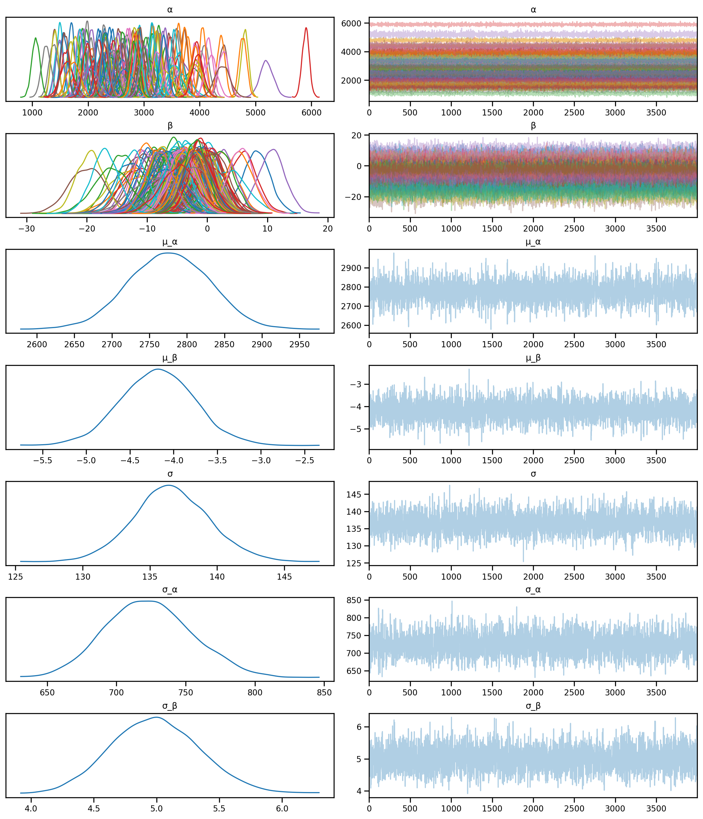

predictive_hierarchical = Predictive(final_model, mcmc_final.get_samples())

predictions_train_hierarchical = predictive_hierarchical(rng_key,
                                                         sample_weeks = model_kwargs["sample_weeks"],
                                                         sample_patient_code = model_kwargs["sample_patient_code"])['fvc']

mu_predictions_train_h = predictions_train_hierarchical.mean(axis=0)
std_predictions_train_h = predictions_train_hierarchical.std(axis=0)

maes["Hierarchical"] = mean_absolute_error(sample_fvc, mu_predictions_train_h)

coverages["Hierarchical"] = coverage(sample_fvc, mu_predictions_train_h, std_predictions_train_h).item()

print(maes)
print(coverages)

{'LinearRegression': 654.8103093180237, 'PooledModel': 654.6283571306085, 'UnpooledModel': 98.18583518632232, 'UnpooledModel2': 81.93005607511398, 'Hierarchical': 83.05726212759492}
{'pooled': 0.9399612545967102, 'unpooled': 0.974822461605072, 'unpooled2': 0.886378288269043, 'Hierarchical': 0.9754680395126343}

pd.Series(maes)

LinearRegression    654.810309
PooledModel         654.628357
UnpooledModel        98.185835
UnpooledModel2       81.930056
Hierarchical         83.057262
dtype: float64

# Predict for a given patient


def predict_final(patient_code):
    predictions = predictive_final(rng_key, all_weeks, patient_code)
    mu = predictions["fvc"].mean(axis=0)
    sigma = predictions["fvc"].std(axis=0)
    return mu, sigma

# Plot the predictions for a given patient
def plot_patient_final(patient_code):
    mu, sigma = predict_final(patient_code)
    plt.plot(all_weeks, mu)
    plt.fill_between(all_weeks, mu - sigma, mu + sigma, alpha=0.1)
    id_to_patient = patient_encoder.inverse_transform([patient_code])[0]
    #print(id_to_patient[0], patient_code)
    #print(patient_code, id_to_patient)
    patient_weeks = train[train["Patient"] == id_to_patient]["Weeks"]
    patient_fvc = train[train["Patient"] == id_to_patient]["FVC"]
    plt.scatter(patient_weeks, patient_fvc, alpha=0.5)
    #plt.scatter(sample_weeks[train["patient_code"] == patient_code.item()], fvc[train["patient_code"] == patient_code.item()], alpha=0.5)
    plt.xlabel("Weeks")
    plt.ylabel("FVC")
    plt.title(patient_encoder.inverse_transform([patient_code])[0])

# plot for a given patient
plot_patient_final(np.array([0]))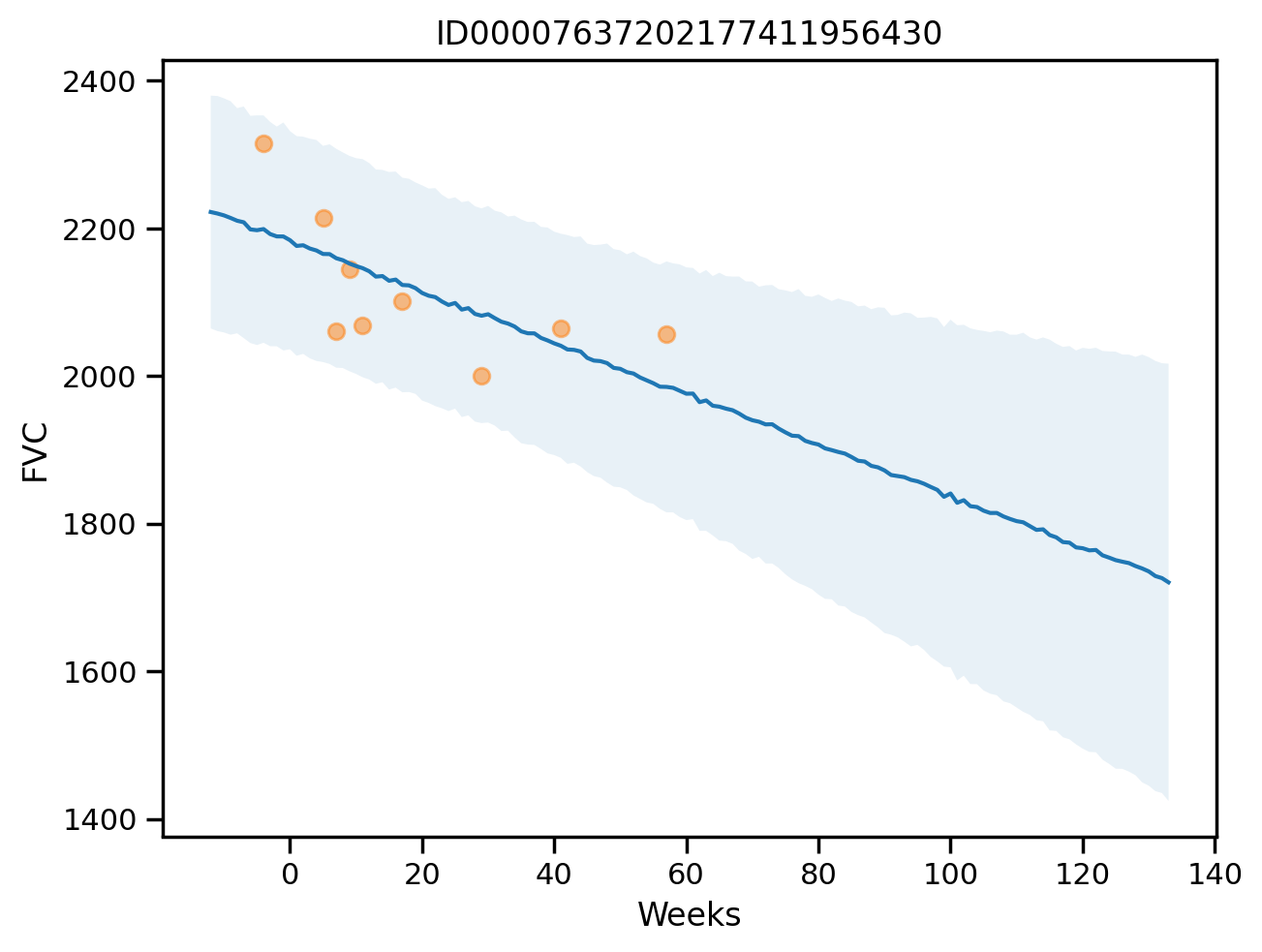

plot_total(0)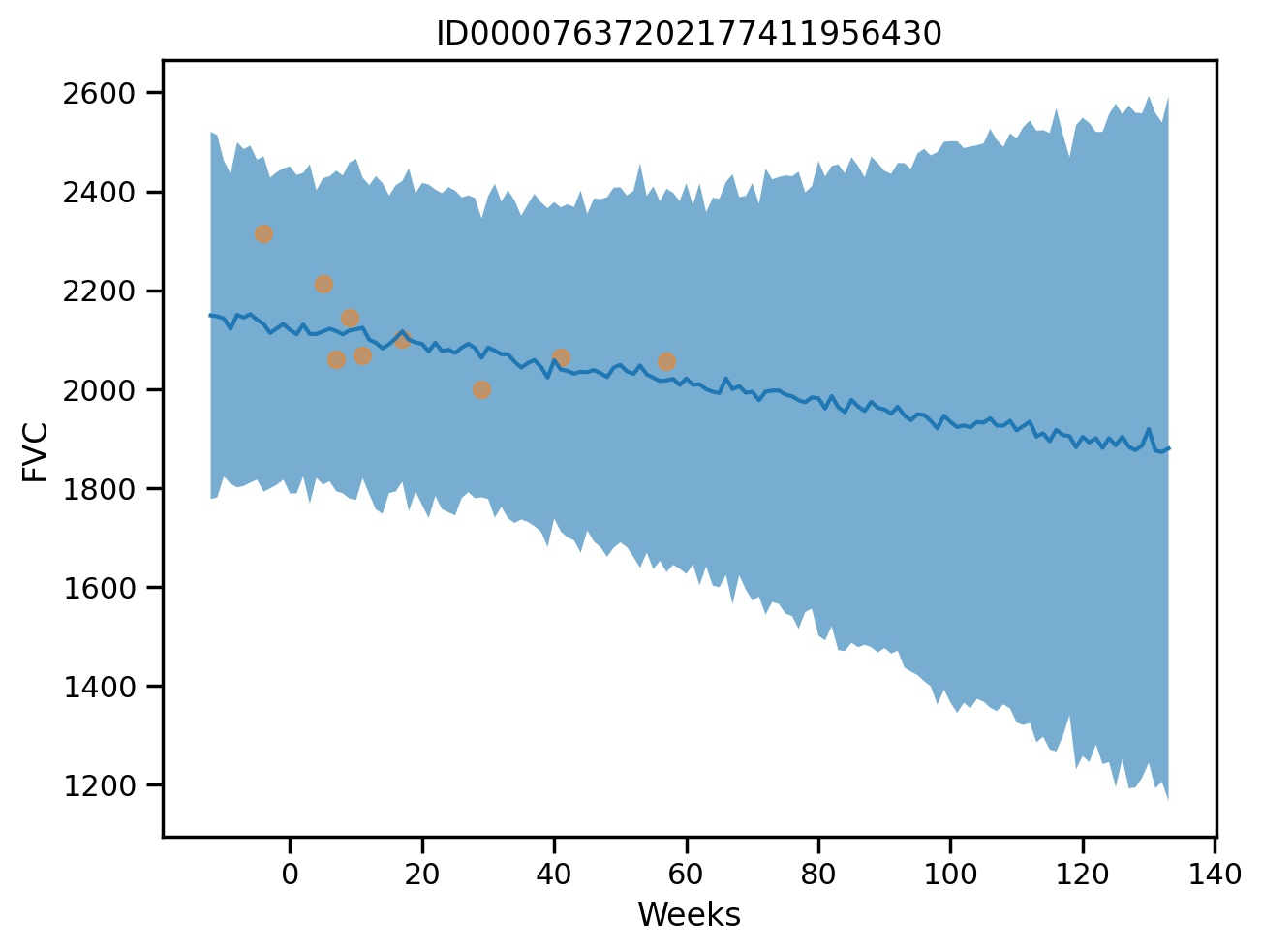

Questions to ponder

• Incorporating extra information
• How to get sigma for sklearn model
• How to predict for a new partipant in the hierarchical model
  • Assuming they have some observations
    • Add the data from this participant at the training time
    • “Fine-tune” on this participant data
  • Assuming they do not have any observations