import torch
import numpy as np
import matplotlib.pyplot as plt
import pandas as pd
import matplotlib.pyplot as plt
import seaborn as sns
%matplotlib inline
# Retina display
%config InlineBackend.figure_format = 'retina'
import warnings
warnings.filterwarnings('ignore')

from tueplots import bundles
plt.rcParams.update(bundles.beamer_moml())


# Also add despine to the bundle using rcParams
plt.rcParams['axes.spines.right'] = False
plt.rcParams['axes.spines.top'] = False

# Increase font size to match Beamer template
plt.rcParams['font.size'] = 16
# Make background transparent
plt.rcParams['figure.facecolor'] = 'none'

true_pi = torch.pi
true_pi

3.141592653589793

import torch
import torch.distributions as dist

def estimate_pi(N, seed):
    torch.manual_seed(seed)
    xy = torch.rand(N, 2)  # Generate N random points in [0, 1] × [0, 1]
    distance = torch.sqrt(xy[:, 0]**2 + xy[:, 1]**2)  # Calculate distance from the origin
    inside_circle = distance <= 1.0  # Check if point falls inside the quarter circle
    points_inside = torch.sum(inside_circle).item()  # Count points inside the quarter circle
    pi_estimate = (points_inside / N) * 4.0  # Calculate the π estimate
    return pi_estimate

N = 10000
seed = 42
torch.manual_seed(seed)
xy = torch.rand(N, 2) 
x1 = xy[:, 0]
x2 = xy[:, 1]

distances = torch.sqrt(x1**2 + x2**2)

c = distances <= 1.0

plt.scatter(x1, x2, c = c.float())
plt.gca().set_aspect('equal')

plt.title((c.sum().item()/N)*4)

Text(0.5, 1.0, '3.1464')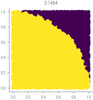

# Different random seeds and sample sizes
random_seeds = [0, 1, 2, 3, 4, 5]
log_sample_sizes = [1, 2, 3, 4, 5, 6, 7, 8]
sample_sizes = [10**i for i in log_sample_sizes]

pi_estimates = []
for seed in random_seeds:
    for N in sample_sizes:
        pi_estimate = estimate_pi(N, seed)
        pi_estimates.append((seed, N, pi_estimate))

	seed	N	pi_estimate
0	0	10	3.200000
1	0	100	3.200000
2	0	1000	3.140000
3	0	10000	3.139200
4	0	100000	3.137200
5	0	1000000	3.140544
6	0	10000000	3.141136
7	0	100000000	3.141476
8	1	10	3.600000
9	1	100	2.880000

# Create a Pandas DataFrame from the list of tuples
df = pd.DataFrame(pi_estimates, columns=["seed", "N", "pi_estimate"])
df.head(20)

	seed	N	pi_estimate
0	0	10	3.200000
1	0	100	3.200000
2	0	1000	3.140000
3	0	10000	3.139200
4	0	100000	3.137200
5	0	1000000	3.140544
6	0	10000000	3.141136
7	0	100000000	3.141476
8	1	10	3.600000
9	1	100	2.880000
10	1	1000	3.096000
11	1	10000	3.144000
12	1	100000	3.139640
13	1	1000000	3.143724
14	1	10000000	3.142105
15	1	100000000	3.141681
16	2	10	3.600000
17	2	100	3.120000
18	2	1000	3.140000
19	2	10000	3.144000

df_grouped = df.groupby("N").agg(["mean", "std"])["pi_estimate"]
df_grouped

	mean	std
N
10	3.200000	0.357771
100	3.120000	0.153883
1000	3.147333	0.090099
10000	3.147200	0.007065
100000	3.140580	0.007081
1000000	3.142121	0.001377
10000000	3.141548	0.000712
100000000	3.141659	0.000162

# Plot the estimates using mean and standard deviation
plt.figure(figsize=(8, 6))
df_grouped["mean"].plot(yerr=df_grouped["std"], capsize=5, marker="o")
plt.axhline(true_pi, color="black", linestyle="--")
plt.xlabel("Sample Size")
plt.ylabel("Estimated π")
plt.title("Estimating π using Monte Carlo Sampling")
# log scale on x-axis
plt.xscale("log")

findfont: Font family ['cursive'] not found. Falling back to DejaVu Sans.
findfont: Generic family 'cursive' not found because none of the following families were found: Apple Chancery, Textile, Zapf Chancery, Sand, Script MT, Felipa, Comic Neue, Comic Sans MS, cursive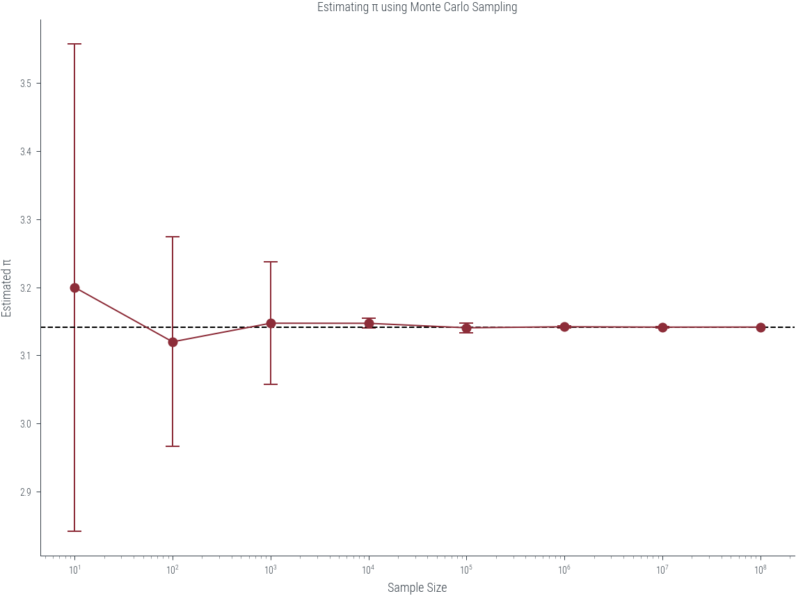

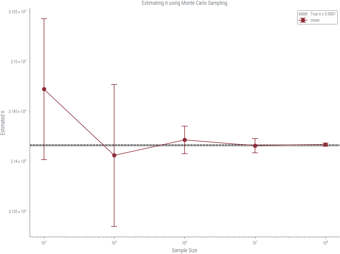
# Plot only 10^4 and higher
plt.figure(figsize=(8, 6))
subset = df_grouped.query("N >= 10**4")
subset["mean"].plot(yerr=subset["std"], capsize=5, marker="o")
plt.xlabel("Sample Size")
plt.ylabel("Estimated π")
plt.title("Estimating π using Monte Carlo Sampling")
# log scale on x-axis
plt.xscale("log")
plt.yscale("log")

plt.axhline(true_pi, color="black", linestyle="--")

# plot true_pi +- 0.0001
plt.axhspan(true_pi - 0.0001, true_pi + 0.0001, color="black", alpha=0.2, label="True π ± 0.0001")
plt.legend()

<matplotlib.legend.Legend at 0x7f6b93cb3d90>