Probabilistic Machine Learning

import torch
import numpy as np
import matplotlib.pyplot as plt
import pandas as pd
import matplotlib.pyplot as plt
%matplotlib inline
# Retina display
%config InlineBackend.figure_format = 'retina'

from tueplots import bundles
plt.rcParams.update(bundles.beamer_moml())


# Also add despine to the bundle using rcParams
plt.rcParams['axes.spines.right'] = False
plt.rcParams['axes.spines.top'] = False

# Increase font size to match Beamer template
plt.rcParams['font.size'] = 16
# Make background transparent
plt.rcParams['figure.facecolor'] = 'none'

c1 = torch.distributions.Normal(80, 10)
c2 = torch.distributions.Normal(70, 10)
c3 = torch.distributions.Normal(90, 5)

# Plot the distributions
x = torch.linspace(0, 105, 1000)
plt.plot(x, c1.log_prob(x).exp(), label='C1')
plt.plot(x, c2.log_prob(x).exp(), label='C2')
plt.plot(x, c3.log_prob(x).exp(), label='C3')
# Fill the area under the curve
plt.fill_between(x, c1.log_prob(x).exp(), alpha=0.2)
plt.fill_between(x, c2.log_prob(x).exp(), alpha=0.2)
plt.fill_between(x, c3.log_prob(x).exp(), alpha=0.2)

plt.xlabel('Marks')
plt.ylabel('Probability')

plt.legend(title='Class')
plt.savefig('../figures/mle/mle-example.pdf', bbox_inches='tight')

# Vertical line at x = 85
marks = torch.tensor([82.])
plt.axvline(marks.item(), color='k', linestyle='--', lw=2)
# Draw horizontal line to show the probability at x = 85
plt.hlines(c1.log_prob(marks).exp(), 0, marks.item(), color='C0', linestyle='--', lw=2)
plt.hlines(c2.log_prob(marks).exp(), 0, marks.item(), color='C1', linestyle='--', lw=2)
plt.hlines(c3.log_prob(marks).exp(), 0, marks.item(), color='C2', linestyle='--', lw=2)
plt.savefig('../figures/mle/mle-example-2.pdf', bbox_inches='tight')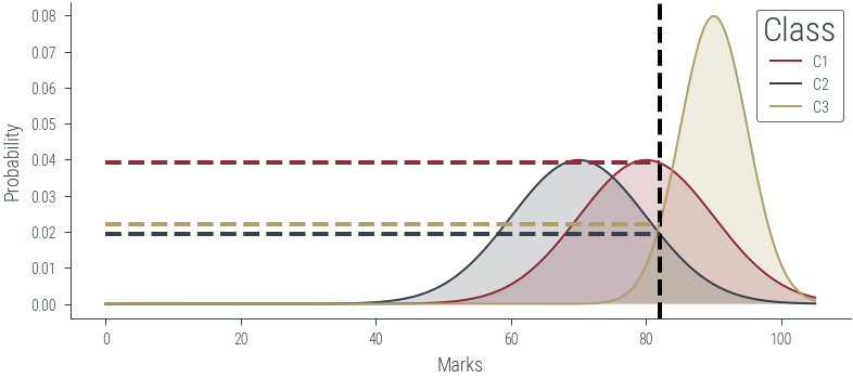

obs = torch.tensor([20.0])
sigma = torch.tensor([1.0])

# Plot the likelihood
mus = torch.linspace(0, 40, 1000)
plt.plot(mus, torch.distributions.Normal(mus, sigma).log_prob(obs).exp())
plt.xlabel(r'Parameter ($\mu$)')
plt.ylabel(r'Likelihood $p(x = 20|\mu$)')

Text(0, 0.5, 'Likelihood $p(x = 20|\\mu$)')

findfont: Font family ['cursive'] not found. Falling back to DejaVu Sans.
findfont: Generic family 'cursive' not found because none of the following families were found: Apple Chancery, Textile, Zapf Chancery, Sand, Script MT, Felipa, Comic Neue, Comic Sans MS, cursive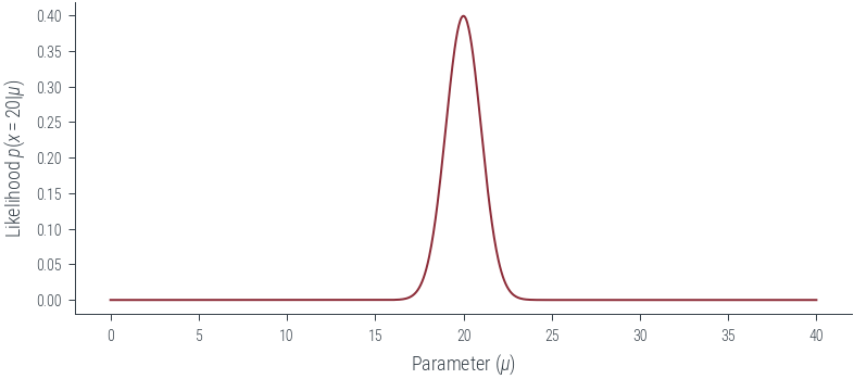

from ipywidgets import interact, interactive, fixed, interact_manual
import ipywidgets as widgets

# Interactive plot showing fitting normal distribution of varying mu to one data point

def plot_norm(mu):
    mu = torch.tensor(mu)
    sigma = torch.tensor(1.0)
    x = torch.tensor(20.0)
    n = torch.distributions.Normal(mu, sigma)
    x_lin = torch.linspace(0, 40, 500)
    y_lin = n.log_prob(x_lin).exp()
    likelihood = n.log_prob(x).exp()
    plt.plot(x_lin, y_lin, label=rf"$\mathcal{{N}}({mu.item():0.4f}, 1)$")
    plt.legend()
    plt.title(f"Likelihood={likelihood:.4f}")
    plt.ylim(0, 0.5)
    plt.fill_between(x_lin, y_lin, alpha=0.2)
    plt.axvline(x=x, color="black", linestyle="--")
    plt.axhline(y=likelihood, color="black", linestyle="--")
        
#plot_norm(20)
interact(plot_norm, mu=(0, 30, 0.1))

<function __main__.plot_norm(mu)>

# Interactive plot showing fitting normal distribution of varying mu to one data point

def plot_norm_log(mu):
    mu = torch.tensor(mu)
    sigma = torch.tensor(1.0)
    x = torch.tensor(20.0)
    n = torch.distributions.Normal(mu, sigma)
    x_lin = torch.linspace(0, 40, 500)
    fig, ax = plt.subplots(nrows=2, sharex=True)
    y_log_lin = n.log_prob(x_lin)
    y_lin = y_log_lin.exp()
    ll = n.log_prob(x)
    likelihood = ll.exp()
    ax[0].plot(x_lin, y_lin, label=rf"$\mathcal{{N}}({mu.item():0.4f}, 1)$")
    #plt.legend()
    ax[0].set_title(f"Likelihood={likelihood:.4f}")
    ax[0].set_ylim(0, 0.5)
    ax[0].fill_between(x_lin, y_lin, alpha=0.2)

    ax[1].plot(x_lin, y_log_lin, label=rf"$\mathcal{{N}}({mu.item():0.4f}, 1)$")
    ax[1].set_title(f"Log Likelihood={ll:.4f}")
    ax[1].set_ylim(-500, 20)
    
    ax[0].axvline(x=x, color="black", linestyle="--")
    ax[0].axhline(y=likelihood, color="black", linestyle="--")

    ax[1].axvline(x=x, color="black", linestyle="--")
    ax[1].axhline(y=ll, color="black", linestyle="--")
        
#plot_norm_log(10)
interact(plot_norm_log, mu=(0, 30, 0.1))

<function __main__.plot_norm_log(mu)>

# Plot the distributions
def plot_class(class_num):
    x = torch.linspace(0, 105, 1000)
    dist = [c1, c2, c3][class_num-1]
    plt.plot(x, dist.log_prob(x).exp(), label=f'C{class_num}')
    plt.fill_between(x, dist.log_prob(x).exp(), alpha=0.2)


    plt.xlabel('Marks')
    plt.ylabel('Probability')

    #plt.legend(title='Class')
    #plt.savefig('../figures/mle/mle-example.pdf', bbox_inches='tight')

    # Vertical line at x = 82
    marks = torch.tensor([82., 72.0])
    for mark in marks:
        plt.axvline(mark.item(), color='k', linestyle='--', lw=2)

        plt.hlines(dist.log_prob(mark).exp(), 0, mark.item(), color='C0', linestyle='--', lw=2, label=f"P({mark.item()}|Class ={dist.log_prob(mark).exp().item():0.4f}")
        #plt.hlines(c2.log_prob(mark).exp(), 0, mark.item(), color='C1', linestyle='--', lw=2)
        #plt.hlines(c3.log_prob(mark).exp(), 0, mark.item(), color='C2', linestyle='--', lw=2)
    #plt.savefig('../figures/mle/mle-example-2.pdf', bbox_inches='tight')
    plt.legend()
    #plt.savefig("..")

plot_class(1)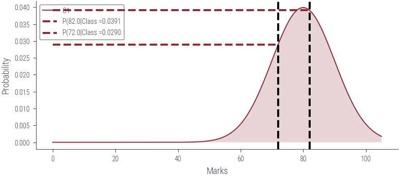

plot_class(2)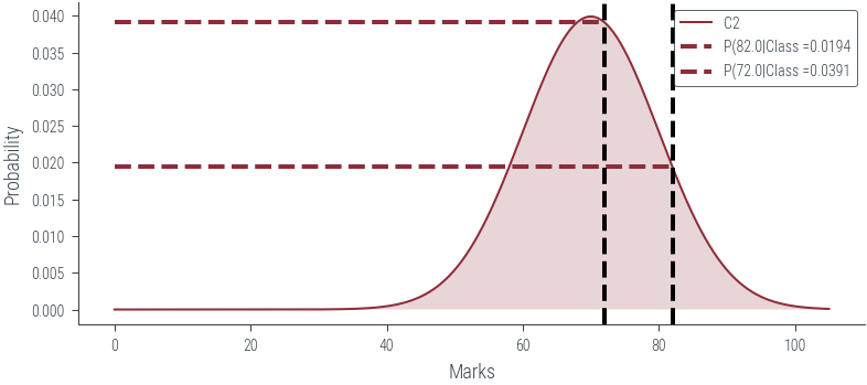

plot_class(3)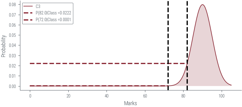

#
s1 = torch.tensor([82.0])
s2 = torch.tensor([72.0])

p_s1_c1 = c1.log_prob(s1).exp()
p_s1_c2 = c2.log_prob(s1).exp()
p_s1_c3 = c3.log_prob(s1).exp()

p_s2_c1 = c1.log_prob(s2).exp()
p_s2_c2 = c2.log_prob(s2).exp()
p_s2_c3 = c3.log_prob(s2).exp()

# Create dataframe
df = pd.DataFrame({
    'Class': ['C1', 'C2', 'C3'],
    'Student 1 (82)': [p_s1_c1.item(), p_s1_c2.item(), p_s1_c3.item()],
    'Student 2 (72)': [p_s2_c1.item(), p_s2_c2.item(), p_s2_c3.item()]
})

df = df.set_index('Class')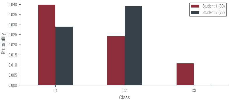
df

	Student 1 (82)	Student 2 (72)
Class
C1	0.039104	0.028969
C2	0.019419	0.039104
C3	0.022184	0.000122

df.plot(kind='bar', rot=0)

<AxesSubplot:xlabel='Class'>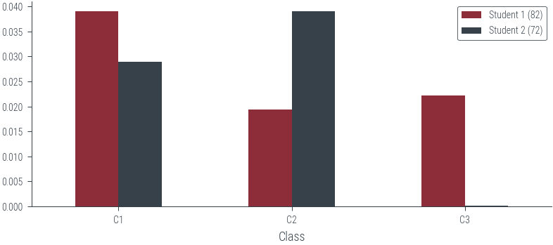

# Multiply the probabilities
df.aggregate('prod', axis=1)

Class
C1    0.001133
C2    0.000759
C3    0.000003
dtype: float64

df.aggregate('prod', axis=1).plot(kind='bar', rot=0)

<AxesSubplot:xlabel='Class'>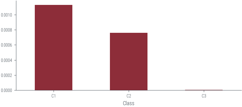

# Create a slider to change s1 and s2 marks and plot the likelihood


def plot_likelihood(s1, s2, scale='log'):
    s1 = torch.tensor([s1])
    s2 = torch.tensor([s2])
    p_s1_c1 = c1.log_prob(s1)
    p_s1_c2 = c2.log_prob(s1)
    p_s1_c3 = c3.log_prob(s1)

    p_s2_c1 = c1.log_prob(s2)
    p_s2_c2 = c2.log_prob(s2)
    p_s2_c3 = c3.log_prob(s2)


    # Create dataframe
    df = pd.DataFrame({
        'Class': ['C1', 'C2', 'C3'],
        f'Student 1 ({s1.item()})': [p_s1_c1.item(), p_s1_c2.item(), p_s1_c3.item()],
        f'Student 2 ({s2.item()})': [p_s2_c1.item(), p_s2_c2.item(), p_s2_c3.item()]
    })
    
    

    df = df.set_index('Class')
    if scale!='log':
        df  = df.apply(np.exp)
    df.plot(kind='bar', rot=0)
    plt.ylabel('Probability')
    plt.xlabel('Class')

    if scale=='log':
        plt.ylabel('Log Probability')
        #plt.yscale('log')

plot_likelihood(80, 72, scale='linear')

plot_likelihood(80, 72, scale='log')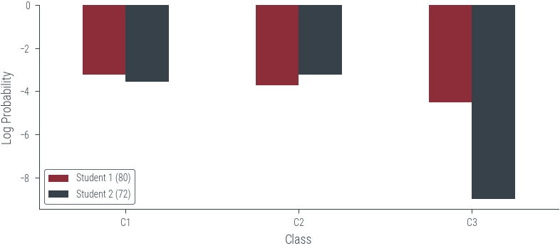

# Interactive plot
interact(plot_likelihood, s1=(0, 100), s2=(0, 100), scale=['linear', 'log'])

<function __main__.plot_likelihood(s1, s2, scale='log')>

# Let us now consider some N points from a univariate Gaussian distribution with mean 0 and variance 1.

N = 50
torch.manual_seed(2)
samples = torch.distributions.Normal(0, 1).sample((N,))
samples
samples.mean(), samples.std(correction=0)

(tensor(-0.0089), tensor(1.0376))

plt.scatter(samples, np.zeros_like(samples))

<matplotlib.collections.PathCollection at 0x7f93d6f98550>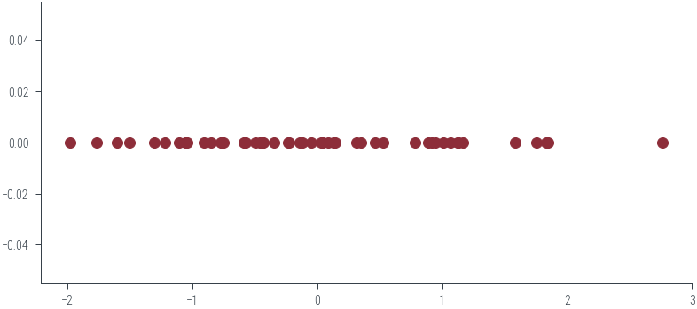

dist = torch.distributions.Normal(0, 1)
dist.log_prob(samples)

tensor([-1.4606, -1.3390, -1.7694, -1.5346, -1.6616, -1.6006, -1.4780, -0.9260,
        -1.3310, -0.9785, -1.0821, -0.9466, -1.4266, -1.2024, -0.9443, -1.0125,
        -2.0547, -1.0241, -1.2785, -1.0576, -0.9194, -0.9202, -1.4861, -1.3115,
        -1.0266, -1.0433, -0.9272, -4.7362, -0.9288, -1.5451, -0.9686, -2.4551,
        -1.2115, -2.5932, -2.2046, -2.6290, -0.9199, -2.1755, -1.0937, -1.5588,
        -1.3670, -2.4799, -1.0891, -1.0160, -2.8774, -1.2221, -1.2191, -0.9287,
        -0.9790, -0.9227])

def ll(mu, sigma):
    mu = torch.tensor(mu)
    sigma = torch.tensor(sigma)

    dist = torch.distributions.Normal(mu, sigma)
    loglik = dist.log_prob(samples).sum()
    return dist, loglik

def plot_normal(mu, sigma):
    xs = torch.linspace(-5, 5, 100)
    dist, loglik = ll(mu, sigma)
    ys_log = dist.log_prob(xs)
    plt.plot(xs, ys_log)

    plt.scatter(samples, dist.log_prob(samples), color='C3', alpha=0.5)
    plt.title(f'log likelihood: {loglik:.8f}')

plot_normal(0, 1)
#plt.ylim(-1.7, -1.6)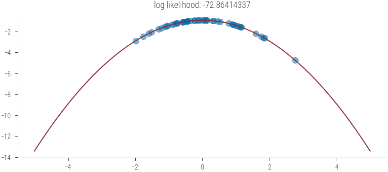

interact(plot_normal, mu=(-3.0, 3.0), sigma=(0.1, 10))

<function __main__.plot_normal(mu, sigma)>

def get_lls(mus, sigmas):

    lls = torch.zeros((len(mus), len(sigmas)))
    for i, mu in enumerate(mus):
        for j, sigma in enumerate(sigmas):

            lls[i, j] = ll(mu, sigma)[1]
    return lls

mus = torch.linspace(-1, 1, 100)
sigmas = torch.linspace(0.1, 1.5, 100)
lls = get_lls(mus, sigmas)

/tmp/ipykernel_444491/3787141935.py:2: UserWarning: To copy construct from a tensor, it is recommended to use sourceTensor.clone().detach() or sourceTensor.clone().detach().requires_grad_(True), rather than torch.tensor(sourceTensor).
  mu = torch.tensor(mu)
/tmp/ipykernel_444491/3787141935.py:3: UserWarning: To copy construct from a tensor, it is recommended to use sourceTensor.clone().detach() or sourceTensor.clone().detach().requires_grad_(True), rather than torch.tensor(sourceTensor).
  sigma = torch.tensor(sigma)

pd.DataFrame(lls.numpy(), index=mus.numpy(), columns=sigmas.numpy())

	0.100000	0.114141	0.128283	0.142424	0.156566	0.170707	0.184848	0.198990	0.213131	0.227273	...	1.372727	1.386869	1.401010	1.415151	1.429293	1.443434	1.457576	1.471717	1.485859	1.500000
-1.000000	-5077.877930	-3888.119141	-3070.949951	-2485.914551	-2052.976318	-1723.822998	-1467.891479	-1265.083740	-1101.745483	-968.337524	...	-89.101242	-89.059502	-89.029251	-89.009949	-89.001060	-89.002075	-89.012505	-89.031929	-89.059898	-89.096008
-0.979798	-4978.790039	-3812.062744	-3010.738281	-2437.065918	-2012.553467	-1689.820068	-1438.892090	-1240.059692	-1079.932007	-949.154175	...	-88.575401	-88.544327	-88.524429	-88.515175	-88.516029	-88.526489	-88.546104	-88.574448	-88.611084	-88.655617
-0.959596	-4881.743652	-3737.573975	-2951.766602	-2389.223145	-1972.963379	-1656.517456	-1410.490112	-1215.551025	-1058.567871	-930.365845	...	-88.060394	-88.039780	-88.030014	-88.030586	-88.040977	-88.060699	-88.089317	-88.126389	-88.171516	-88.224297
-0.939394	-4786.737305	-3664.650146	-2894.034424	-2342.386963	-1934.205566	-1623.915161	-1382.685181	-1191.557739	-1037.652710	-911.972656	...	-87.556213	-87.545830	-87.545990	-87.556183	-87.575905	-87.604698	-87.642128	-87.687759	-87.741196	-87.802048
-0.919192	-4693.770996	-3593.292969	-2837.542480	-2296.556152	-1896.280029	-1592.012939	-1355.477539	-1168.079590	-1017.187012	-893.974426	...	-87.062874	-87.062485	-87.072350	-87.091965	-87.120834	-87.158508	-87.204544	-87.258545	-87.320107	-87.388863
...	...	...	...	...	...	...	...	...	...	...	...	...	...	...	...	...	...	...	...	...	...
0.919192	-4775.875488	-3656.313477	-2887.434814	-2337.032471	-1929.774536	-1620.187744	-1379.506714	-1188.814819	-1035.261719	-909.869873	...	-87.498581	-87.489357	-87.490654	-87.501953	-87.522743	-87.552574	-87.591011	-87.637611	-87.691994	-87.753777
0.939394	-4870.645508	-3729.055664	-2945.022949	-2383.752197	-1968.436035	-1652.709229	-1407.242188	-1212.748413	-1056.124878	-928.217346	...	-88.001511	-87.982071	-87.973473	-87.975166	-87.986656	-88.007431	-88.037086	-88.075157	-88.121246	-88.174980
0.959596	-4967.457520	-3803.364014	-3003.851562	-2431.478760	-2007.930176	-1685.930908	-1435.575439	-1237.197510	-1077.437134	-946.959961	...	-88.515259	-88.485413	-88.466705	-88.458580	-88.460556	-88.472092	-88.492760	-88.522125	-88.559746	-88.605247
0.979798	-5066.307617	-3879.238281	-3063.919678	-2480.210938	-2048.256348	-1719.852661	-1464.505371	-1262.161865	-1099.198608	-966.097595	...	-89.039841	-88.999352	-88.970322	-88.952187	-88.944420	-88.946533	-88.958046	-88.978508	-89.007492	-89.044586
1.000000	-5167.200195	-3956.678955	-3125.228271	-2529.948730	-2089.415527	-1754.474854	-1494.032837	-1287.641602	-1121.409302	-985.630249	...	-89.575256	-89.523895	-89.484329	-89.455971	-89.438293	-89.430779	-89.432945	-89.444313	-89.464470	-89.492989

100 rows × 100 columns

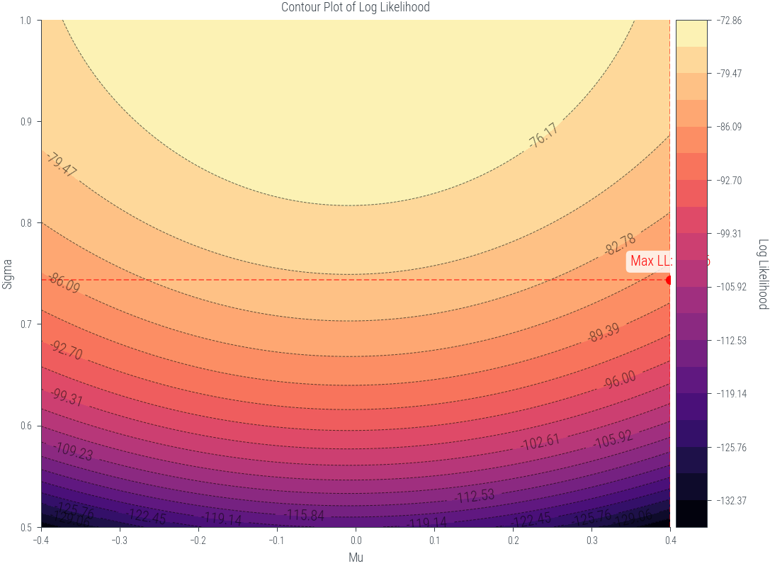
from mpl_toolkits.axes_grid1 import make_axes_locatable

def plot_lls(mus, sigmas, lls):
    fig, ax1 = plt.subplots(figsize=(8, 6))
    
    X, Y = np.meshgrid(mus, sigmas)
    
    max_indices = np.unravel_index(np.argmax(lls), lls.shape)
    max_mu = mus[max_indices[1]]
    max_sigma = sigmas[max_indices[0]]
    max_loglik = lls[max_indices]

    # Define levels with increasing granularity
    levels_low = np.linspace(lls.min(), max_loglik, 20)
    levels_high = np.linspace(max_loglik + 0.001, lls.max(), 10)  # Adding a small value to prevent duplicates
    levels = levels_low
    
    # Plot the contour filled plot
    contour = ax1.contourf(X, Y, lls.T, levels=levels, cmap='magma')
    
    # Plot the contour lines
    contour_lines = ax1.contour(X, Y, lls.T, levels=levels, colors='black', linewidths=0.5, alpha=0.6)
    
    # Add contour labels
    ax1.clabel(contour_lines, inline=True, fontsize=10, colors='black', fmt='%1.2f')
    
    ax1.set_xlabel('Mu')
    ax1.set_ylabel('Sigma')
    ax1.set_title('Contour Plot of Log Likelihood')
    
    # Add maximum log likelihood point as scatter on the contour plot
    ax1.scatter([max_mu], [max_sigma], color='red', marker='o', label='Maximum Log Likelihood')
    ax1.annotate(f'Max LL: {max_loglik:.2f}', (max_mu, max_sigma), textcoords="offset points", xytext=(0,10), ha='center', fontsize=10, color='red', bbox=dict(facecolor='white', alpha=0.8, edgecolor='none', boxstyle='round,pad=0.3'))

    ax1.axvline(max_mu, color='red', linestyle='--', alpha=0.5)
    ax1.axhline(max_sigma, color='red', linestyle='--', alpha=0.5)
    
    # Create colorbar outside the plot
    divider = make_axes_locatable(ax1)
    cax = divider.append_axes("right", size="5%", pad=0.05)
    cbar = plt.colorbar(contour, cax=cax)
    cbar.set_label('Log Likelihood', rotation=270, labelpad=15)
    
    plt.tight_layout()
    plt.show()

plot_lls(mus, sigmas, lls)

/tmp/ipykernel_444491/1128417763.py:44: UserWarning: This figure was using constrained_layout, but that is incompatible with subplots_adjust and/or tight_layout; disabling constrained_layout.
  plt.tight_layout()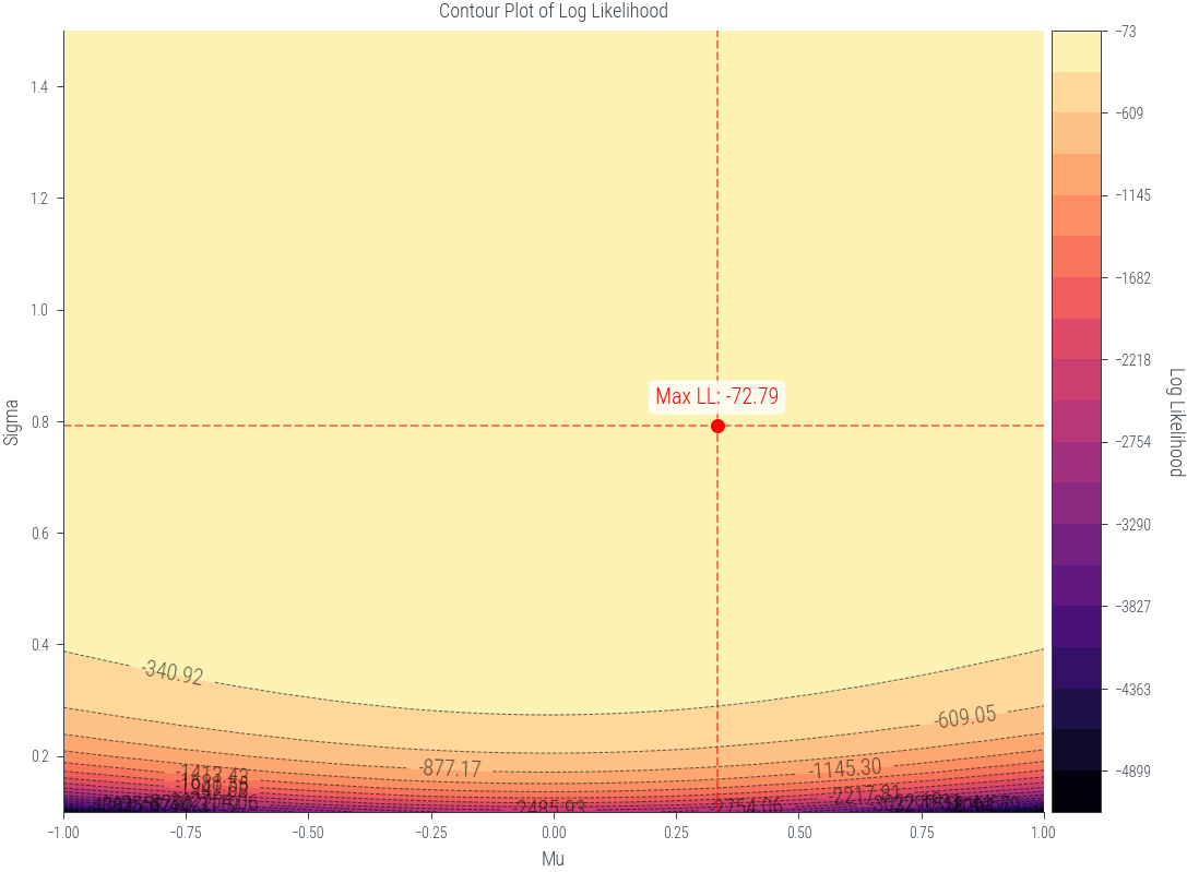

samples.mean(), samples.std(correction=0)

(tensor(-0.0089), tensor(1.0376))

mus = torch.linspace(-0.4, 0.4, 200)
sigmas = torch.linspace(0.5, 1.0,200)
lls = get_lls(mus, sigmas)
plot_lls(mus, sigmas, lls)

/tmp/ipykernel_444491/3787141935.py:2: UserWarning: To copy construct from a tensor, it is recommended to use sourceTensor.clone().detach() or sourceTensor.clone().detach().requires_grad_(True), rather than torch.tensor(sourceTensor).
  mu = torch.tensor(mu)
/tmp/ipykernel_444491/3787141935.py:3: UserWarning: To copy construct from a tensor, it is recommended to use sourceTensor.clone().detach() or sourceTensor.clone().detach().requires_grad_(True), rather than torch.tensor(sourceTensor).
  sigma = torch.tensor(sigma)
/tmp/ipykernel_444491/1128417763.py:44: UserWarning: This figure was using constrained_layout, but that is incompatible with subplots_adjust and/or tight_layout; disabling constrained_layout.
  plt.tight_layout()