Fully Connected PyTorch Visualizer Demo

This notebook turns a small PyTorch dense network into a lecture-style diagram like the hand-drawn sketch.

New capability:

for small fully connected networks, the visualizer can annotate edge weights, node biases, and forward-pass values
if you pass an input_vector, it computes z and a layer by layer

It works for:

nn.Sequential(...) models made of nn.Linear + common activations
custom nn.Module classes that still form a feed-forward fully connected network

It is intentionally not for CNNs, residual blocks, attention, or branching graphs.

import sys
from pathlib import Path

import matplotlib.pyplot as plt
import torch
import torch.nn as nn

torch.manual_seed(7)

repo_root = Path.cwd().resolve()
if repo_root.name == "lecture_demo":
    repo_root = repo_root.parent
if str(repo_root) not in sys.path:
    sys.path.append(str(repo_root))

from fc_model_visualizer import (
    extract_fully_connected_architecture,
    save_figure,
    visualize_fully_connected_model,
)

plt.rcParams["figure.figsize"] = (12, 6)
print(f"Repo root: {repo_root}")
print(f"Torch version: {torch.__version__}")
%config InlineBackend.figure_format = "retina"

Repo root: /Users/nipun/git/principles-ai-teaching
Torch version: 2.9.1

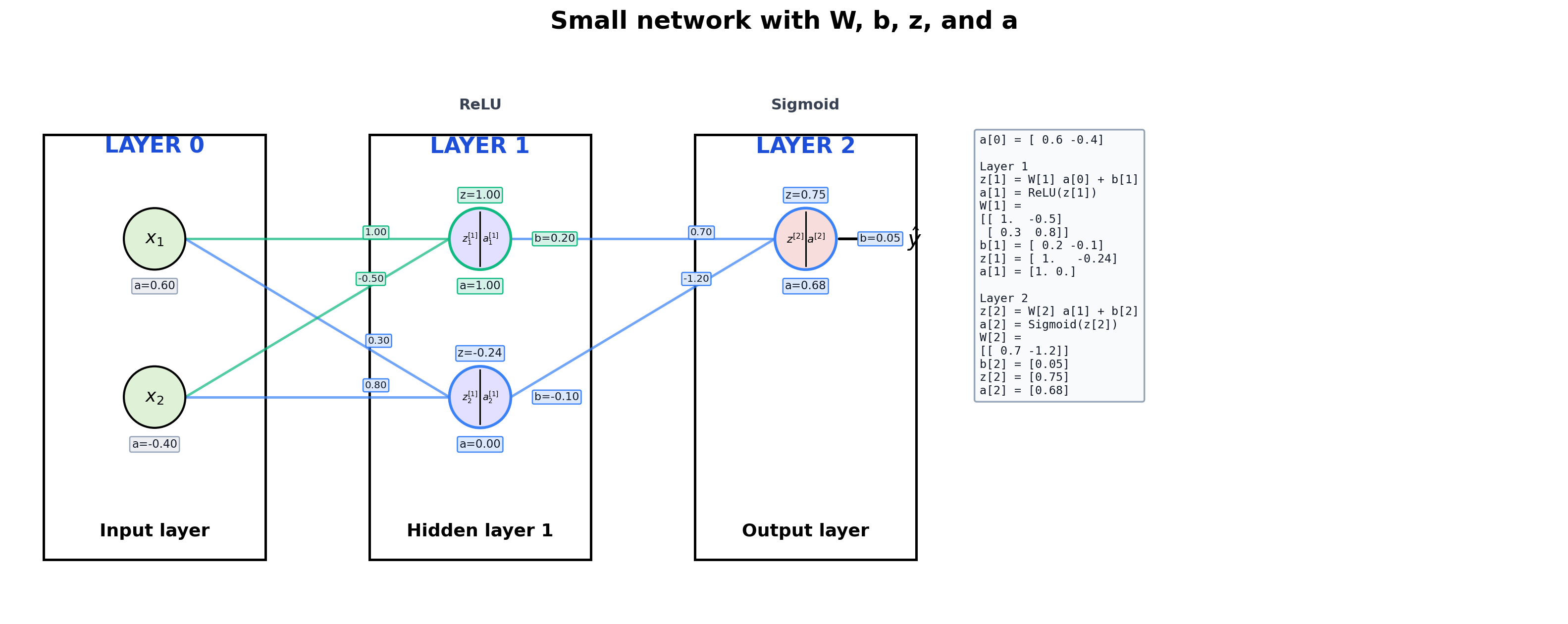
1. Small Network With Full Annotation

This is the best teaching case because we can see everything:

W on the edges
b near each neuron
z = W a + b
a = g(z)
the actual matrix values in a side panel

Design cue:

incoming edges that feed the same neuron share a color
the z, a, and b badges for that neuron use the same accent color

small_model = nn.Sequential(
    nn.Linear(2, 2),
    nn.ReLU(),
    nn.Linear(2, 1),
    nn.Sigmoid(),
)

with torch.no_grad():
    small_model[0].weight.copy_(torch.tensor([[1.0, -0.5], [0.3, 0.8]]))
    small_model[0].bias.copy_(torch.tensor([0.2, -0.1]))
    small_model[2].weight.copy_(torch.tensor([[0.7, -1.2]]))
    small_model[2].bias.copy_(torch.tensor([0.05]))

x_example = torch.tensor([0.6, -0.4], dtype=torch.float32)

print(small_model)
print()
print("Architecture:")
print(extract_fully_connected_architecture(small_model))
print()
print("Input example:", x_example)
print("W[1] =")
print(small_model[0].weight.detach())
print("b[1] =", small_model[0].bias.detach())
print("W[2] =")
print(small_model[2].weight.detach())
print("b[2] =", small_model[2].bias.detach())

Sequential(
  (0): Linear(in_features=2, out_features=2, bias=True)
  (1): ReLU()
  (2): Linear(in_features=2, out_features=1, bias=True)
  (3): Sigmoid()
)

Architecture:
[LinearLayerSpec(in_features=2, out_features=2, activation='ReLU', name='0'), LinearLayerSpec(in_features=2, out_features=1, activation='Sigmoid', name='2')]

Input example: tensor([ 0.6000, -0.4000])
W[1] =
tensor([[ 1.0000, -0.5000],
        [ 0.3000,  0.8000]])
b[1] = tensor([ 0.2000, -0.1000])
W[2] =
tensor([[ 0.7000, -1.2000]])
b[2] = tensor([0.0500])

fig, ax = visualize_fully_connected_model(
    small_model,
    input_labels=[r"$x_1$", r"$x_2$"],
    input_vector=x_example,
    title="Small network with W, b, z, and a",
    max_neurons_per_layer=5,
    show_edge_weights=True,
    show_biases=True,
    show_values=True,
    show_matrix_details=True,
)
plt.show()

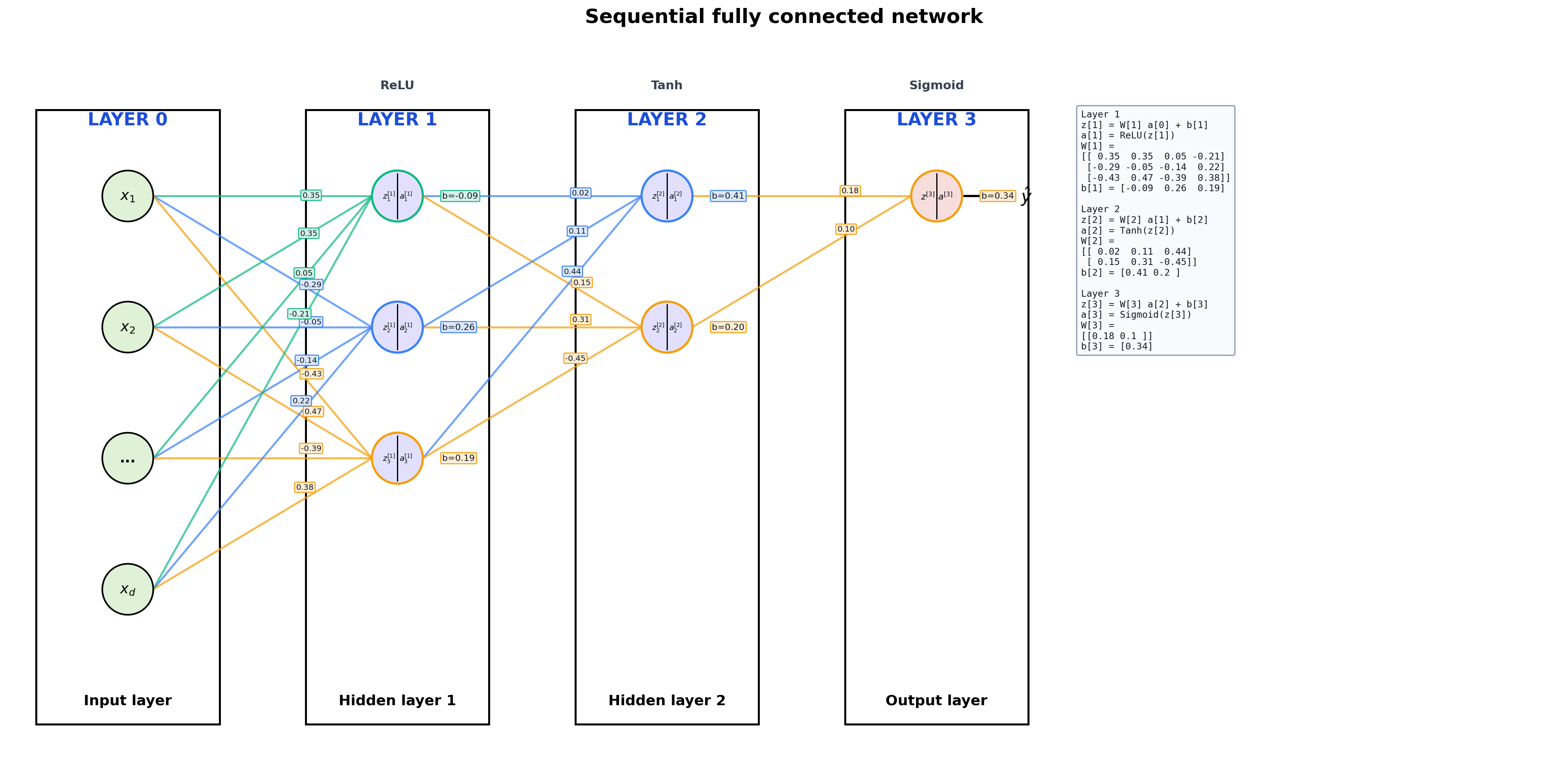
2. A More Typical Sequential Model

The same API works for ordinary lecture examples. It just stops annotating every scalar once the plot would become cluttered.

sequential_model = nn.Sequential(
    nn.Linear(4, 3),
    nn.ReLU(),
    nn.Linear(3, 2),
    nn.Tanh(),
    nn.Linear(2, 1),
    nn.Sigmoid(),
)

print(sequential_model)
print()
print(extract_fully_connected_architecture(sequential_model))

Sequential(
  (0): Linear(in_features=4, out_features=3, bias=True)
  (1): ReLU()
  (2): Linear(in_features=3, out_features=2, bias=True)
  (3): Tanh()
  (4): Linear(in_features=2, out_features=1, bias=True)
  (5): Sigmoid()
)

[LinearLayerSpec(in_features=4, out_features=3, activation='ReLU', name='0'), LinearLayerSpec(in_features=3, out_features=2, activation='Tanh', name='2'), LinearLayerSpec(in_features=2, out_features=1, activation='Sigmoid', name='4')]

fig, ax = visualize_fully_connected_model(
    sequential_model,
    input_labels=[r"$x_1$", r"$x_2$", "...", r"$x_d$"],
    title="Sequential fully connected network",
    max_neurons_per_layer=5,
)
plt.show()

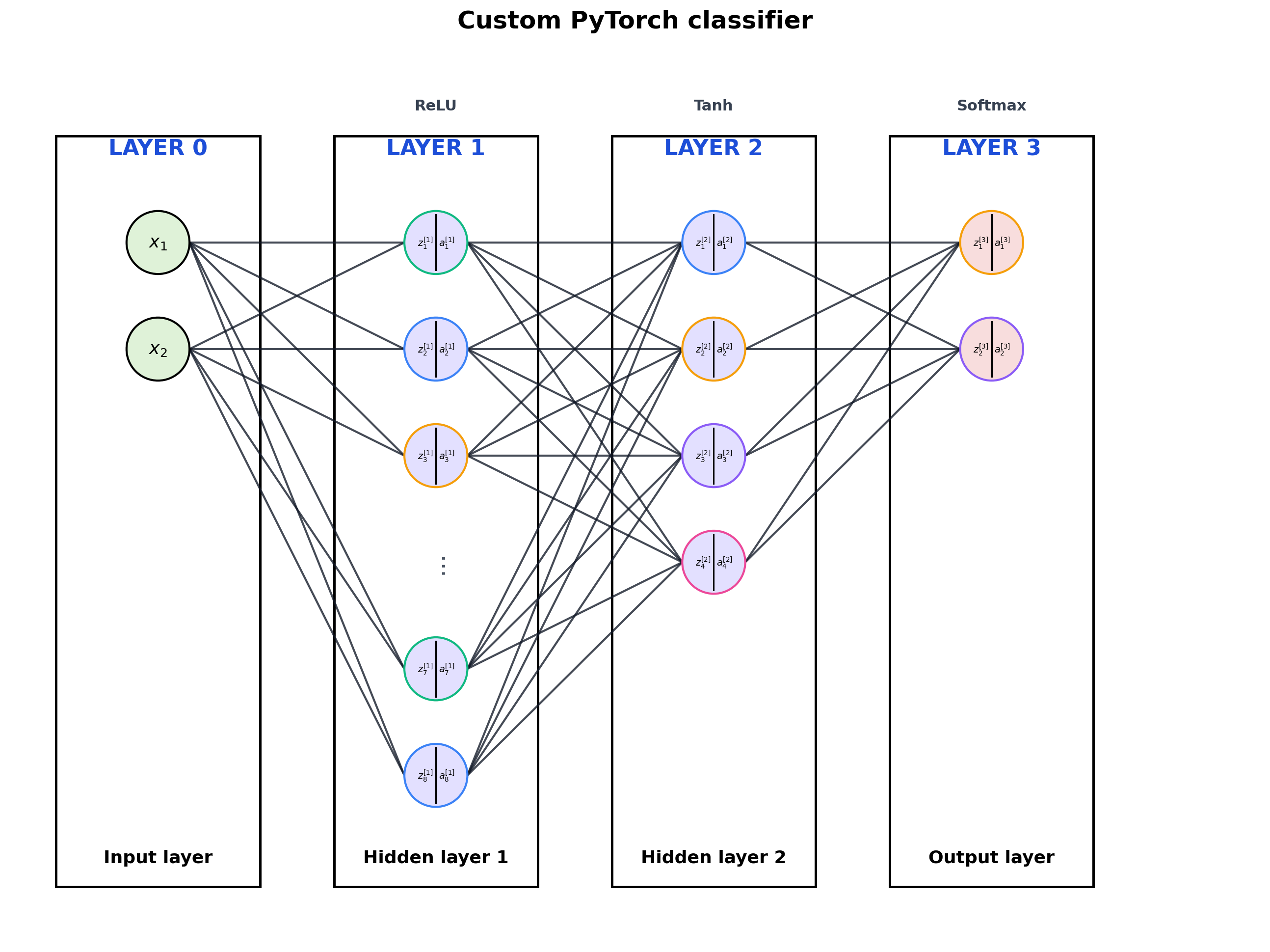
3. Custom `nn.Module`

The visualizer also works when the network is written as a class with named layers.

class SmallClassifier(nn.Module):
    def __init__(self):
        super().__init__()
        self.hidden1 = nn.Linear(2, 8)
        self.hidden2 = nn.Linear(8, 4)
        self.output = nn.Linear(4, 2)

    def forward(self, x):
        x = torch.relu(self.hidden1(x))
        x = torch.tanh(self.hidden2(x))
        return torch.softmax(self.output(x), dim=-1)


custom_model = SmallClassifier()
print(custom_model)
print()
print(extract_fully_connected_architecture(custom_model))

SmallClassifier(
  (hidden1): Linear(in_features=2, out_features=8, bias=True)
  (hidden2): Linear(in_features=8, out_features=4, bias=True)
  (output): Linear(in_features=4, out_features=2, bias=True)
)

[LinearLayerSpec(in_features=2, out_features=8, activation='ReLU', name='hidden1'), LinearLayerSpec(in_features=8, out_features=4, activation='Tanh', name='hidden2'), LinearLayerSpec(in_features=4, out_features=2, activation='Softmax', name='output')]

fig, ax = visualize_fully_connected_model(
    custom_model,
    input_labels=[r"$x_1$", r"$x_2$"],
    output_labels=["class 1", "class 2"],
    title="Custom PyTorch classifier",
    max_neurons_per_layer=6,
)
plt.show()

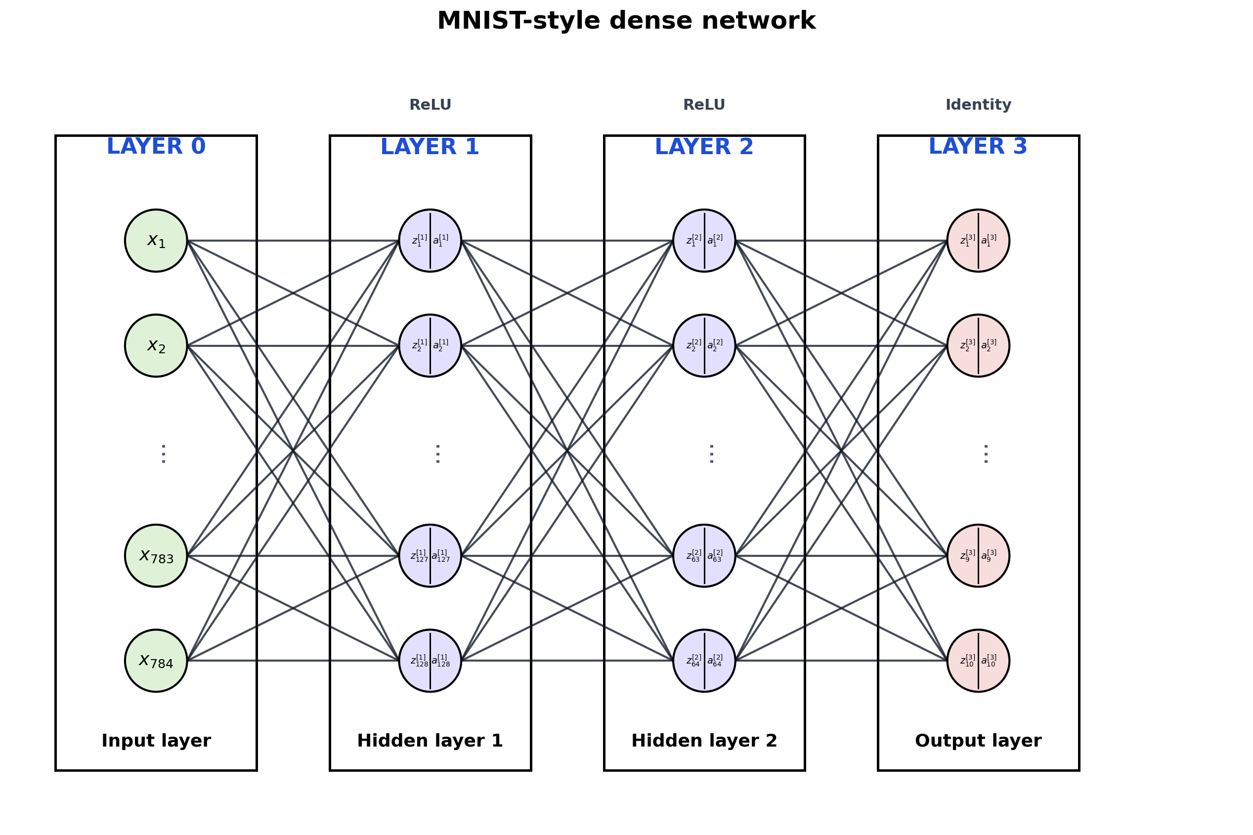
4. Wide Model with Truncation

Large dense layers get summarized with ... so the diagram stays readable.

wide_model = nn.Sequential(
    nn.Linear(784, 128),
    nn.ReLU(),
    nn.Linear(128, 64),
    nn.ReLU(),
    nn.Linear(64, 10),
)

fig, ax = visualize_fully_connected_model(
    wide_model,
    title="MNIST-style dense network",
    max_neurons_per_layer=5,
)
plt.show()

5. Save a Diagram

Reuse the figure in slides or notes by saving PNG and SVG.

output_dir = repo_root / "outputs"
png_path = output_dir / "fc_visualizer_demo.png"
svg_path = output_dir / "fc_visualizer_demo.svg"

fig, ax = visualize_fully_connected_model(
    small_model,
    input_labels=[r"$x_1$", r"$x_2$"],
    input_vector=x_example,
    title="Saved demo network",
    show_edge_weights=True,
    show_biases=True,
    show_values=True,
    show_matrix_details=True,
)
save_figure(fig, png_path=png_path, svg_path=svg_path)

print(f"Saved PNG: {png_path}")
print(f"Saved SVG: {svg_path}")

Saved PNG: /Users/nipun/git/principles-ai-teaching/outputs/fc_visualizer_demo.png
Saved SVG: /Users/nipun/git/principles-ai-teaching/outputs/fc_visualizer_demo.svg

Notes

The visualizer traces the forward graph and looks for:

nn.Linear
activations such as ReLU, Tanh, Sigmoid, Softmax
simple reshaping or flattening operations

Small-network extras:

input_vector=... computes and annotates forward-pass values
show_edge_weights=True writes each scalar weight on its edge
show_biases=True shows each bias near its neuron
show_matrix_details=True adds a side panel with W, b, z, and a