Why Neural Networks Are Powerful

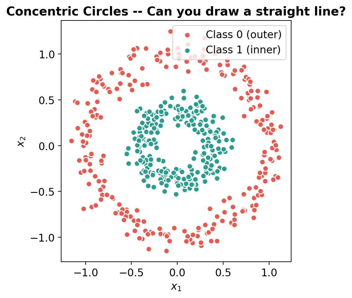
The big idea: Linear models can only draw straight lines. Neural networks can draw any shape.

We’ll prove this step by step, increasing difficulty: 1. Classification (concentric circles) – linear fails, basis expansion works, NN works 2. Regression (sine wave) – same progression, with MSE and R² 3. Harder classification (spirals) – basis expansion breaks down, NN still works 4. Images (MNIST digits) – hand-crafted features vs CNN

At each step: sklearn first, then the same thing in PyTorch, so you see the connection.

import numpy as np
import matplotlib.pyplot as plt
import torch
import torch.nn as nn
import torch.optim as optim
from sklearn.datasets import make_circles
from sklearn.linear_model import LogisticRegression, LinearRegression
from sklearn.preprocessing import PolynomialFeatures
import warnings
warnings.filterwarnings('ignore')

plt.rcParams['figure.figsize'] = (10, 4)
plt.rcParams['font.size'] = 12

# Colors
C0, C1 = '#e85a4f', '#2a9d8f'

print('Ready!')
%config InlineBackend.figure_format = 'retina'

Ready!

def plot_decision_boundary(predict_fn, X, y, title='', ax=None):
    """Plot decision boundary for a classifier."""
    if ax is None:
        fig, ax = plt.subplots(figsize=(5, 5))
    
    # Create mesh
    margin = 0.5
    x_min, x_max = X[:, 0].min() - margin, X[:, 0].max() + margin
    y_min, y_max = X[:, 1].min() - margin, X[:, 1].max() + margin
    xx, yy = np.meshgrid(np.linspace(x_min, x_max, 200),
                         np.linspace(y_min, y_max, 200))
    grid = np.c_[xx.ravel(), yy.ravel()]
    
    Z = predict_fn(grid).reshape(xx.shape)
    
    ax.contourf(xx, yy, Z, levels=[-0.5, 0.5, 1.5], colors=[C0, C1], alpha=0.3)
    ax.contour(xx, yy, Z, levels=[0.5], colors=['black'], linewidths=2)
    
    ax.scatter(X[y == 0, 0], X[y == 0, 1], c=C0, edgecolors='white', s=40, label='Class 0')
    ax.scatter(X[y == 1, 0], X[y == 1, 1], c=C1, edgecolors='white', s=40, label='Class 1')
    ax.set_title(title, fontsize=14, fontweight='bold')
    ax.set_xlabel('$x_1$')
    ax.set_ylabel('$x_2$')
    ax.set_aspect('equal')
    return ax

Part 1: Classification – Concentric Circles

Can you separate inner circle from outer circle with a straight line?

# Generate concentric circles
np.random.seed(42)
X_circles, y_circles = make_circles(n_samples=500, noise=0.08, factor=0.4)

fig, ax = plt.subplots(figsize=(5, 5))
ax.scatter(X_circles[y_circles == 0, 0], X_circles[y_circles == 0, 1], 
           c=C0, edgecolors='white', s=40, label='Class 0 (outer)')
ax.scatter(X_circles[y_circles == 1, 0], X_circles[y_circles == 1, 1], 
           c=C1, edgecolors='white', s=40, label='Class 1 (inner)')
ax.set_title('Concentric Circles -- Can you draw a straight line?', fontsize=14, fontweight='bold')
ax.set_xlabel('$x_1$'); ax.set_ylabel('$x_2$')
ax.legend()
ax.set_aspect('equal')
plt.tight_layout()
plt.show()

Step 1: Logistic Regression (sklearn)

A straight line through this data. Will it work?

# Logistic regression = straight line decision boundary
lr_sklearn = LogisticRegression()
lr_sklearn.fit(X_circles, y_circles)

acc = lr_sklearn.score(X_circles, y_circles)

fig, ax = plt.subplots(figsize=(5, 5))
plot_decision_boundary(lr_sklearn.predict, X_circles, y_circles,
                       f'sklearn Logistic Regression\nAccuracy: {acc:.0%}', ax=ax)
plt.tight_layout()
plt.show()

print(f'Accuracy: {acc:.0%} -- basically random guessing!')
print('A straight line cannot separate circles.')

Accuracy: 50% -- basically random guessing!
A straight line cannot separate circles.

Step 2: Logistic Regression in PyTorch

Same thing, but written in PyTorch. Same result – just to show how PyTorch works.

# Convert data to tensors
X_t = torch.tensor(X_circles, dtype=torch.float32)
y_t = torch.tensor(y_circles, dtype=torch.float32).unsqueeze(1)

# Logistic regression in PyTorch = Linear layer + Sigmoid
torch.manual_seed(42)
logreg_torch = nn.Sequential(
    nn.Linear(2, 1),
    nn.Sigmoid()
)

optimizer = optim.Adam(logreg_torch.parameters(), lr=0.01)
loss_fn = nn.BCELoss()

# Train
losses = []
for epoch in range(500):
    pred = logreg_torch(X_t)
    loss = loss_fn(pred, y_t)
    optimizer.zero_grad()
    loss.backward()
    optimizer.step()
    losses.append(loss.item())

# Predict function for plotting
def predict_logreg_torch(X_np):
    with torch.no_grad():
        probs = logreg_torch(torch.tensor(X_np, dtype=torch.float32))
        return (probs.numpy() > 0.5).astype(int).ravel()

acc = (predict_logreg_torch(X_circles) == y_circles).mean()

fig, axes = plt.subplots(1, 2, figsize=(10, 4.5))
axes[0].plot(losses, color='#1e3a5f')
axes[0].set_xlabel('Epoch'); axes[0].set_ylabel('Loss')
axes[0].set_title('Training Loss', fontweight='bold')

plot_decision_boundary(predict_logreg_torch, X_circles, y_circles,
                       f'PyTorch Logistic Regression\nAccuracy: {acc:.0%}', ax=axes[1])
plt.tight_layout()
plt.show()

print(f'Same result! Accuracy: {acc:.0%}')
print('PyTorch logistic regression = sklearn logistic regression. Both are linear.')

Same result! Accuracy: 50%
PyTorch logistic regression = sklearn logistic regression. Both are linear.

Step 3: Basis Expansion – The Manual Fix

Key idea: The data isn’t linearly separable in \((x_1, x_2)\) space. But what if we add new features?

For circles, the separating boundary is \(x_1^2 + x_2^2 = r^2\). So let’s add \(x_1^2\), \(x_2^2\), \(x_1 x_2\) as features!

This is called basis expansion or feature engineering – we manually create the right features.

# Basis expansion: add polynomial features
poly = PolynomialFeatures(degree=2, include_bias=False)
X_poly = poly.fit_transform(X_circles)

print(f'Original features: {X_circles.shape[1]} -- (x1, x2)')
print(f'After basis expansion: {X_poly.shape[1]} -- ({" , ".join(poly.get_feature_names_out())})')
print()

# sklearn logistic regression on expanded features
lr_poly = LogisticRegression()
lr_poly.fit(X_poly, y_circles)

# For plotting, we need to transform the grid too
def predict_poly_sklearn(X_np):
    return lr_poly.predict(poly.transform(X_np))

acc = lr_poly.score(X_poly, y_circles)

fig, axes = plt.subplots(1, 2, figsize=(10, 4.5))
plot_decision_boundary(lr_sklearn.predict, X_circles, y_circles,
                       f'Without basis expansion\nAccuracy: {lr_sklearn.score(X_circles, y_circles):.0%}', ax=axes[0])
plot_decision_boundary(predict_poly_sklearn, X_circles, y_circles,
                       f'With basis expansion (degree=2)\nAccuracy: {acc:.0%}', ax=axes[1])
plt.tight_layout()
plt.show()

print(f'Accuracy with basis expansion: {acc:.0%}')
print('It works! But we had to KNOW to add x1^2, x2^2, x1*x2.')

Original features: 2 -- (x1, x2)
After basis expansion: 5 -- (x0 , x1 , x0^2 , x0 x1 , x1^2)

Accuracy with basis expansion: 100%
It works! But we had to KNOW to add x1^2, x2^2, x1*x2.

# Same basis expansion, but logistic regression in PyTorch
X_poly_t = torch.tensor(X_poly, dtype=torch.float32)

torch.manual_seed(42)
logreg_poly_torch = nn.Sequential(
    nn.Linear(5, 1),   # 5 features after basis expansion
    nn.Sigmoid()
)

optimizer = optim.Adam(logreg_poly_torch.parameters(), lr=0.01)

for epoch in range(500):
    pred = logreg_poly_torch(X_poly_t)
    loss = loss_fn(pred, y_t)
    optimizer.zero_grad()
    loss.backward()
    optimizer.step()

def predict_poly_torch(X_np):
    with torch.no_grad():
        X_p = torch.tensor(poly.transform(X_np), dtype=torch.float32)
        return (logreg_poly_torch(X_p).numpy() > 0.5).astype(int).ravel()

acc = (predict_poly_torch(X_circles) == y_circles).mean()

fig, ax = plt.subplots(figsize=(5, 5))
plot_decision_boundary(predict_poly_torch, X_circles, y_circles,
                       f'PyTorch + Basis Expansion\nAccuracy: {acc:.0%}', ax=ax)
plt.tight_layout()
plt.show()

print(f'Same idea in PyTorch: {acc:.0%}')

Same idea in PyTorch: 100%

Step 4: Neural Network – No Feature Engineering Needed!

The magic: A neural network on the original 2 features learns its own basis expansion.

No need to manually add \(x_1^2\), \(x_2^2\), etc. The hidden layers figure it out.

# Neural network -- on original (x1, x2) features, NO basis expansion
torch.manual_seed(42)
nn_model = nn.Sequential(
    nn.Linear(2, 16),    # 2 inputs -> 16 hidden neurons
    nn.ReLU(),
    nn.Linear(16, 16),   # 16 -> 16 hidden neurons
    nn.ReLU(),
    nn.Linear(16, 1),    # 16 -> 1 output
    nn.Sigmoid()
)

optimizer = optim.Adam(nn_model.parameters(), lr=0.01)

losses = []
for epoch in range(1000):
    pred = nn_model(X_t)
    loss = loss_fn(pred, y_t)
    optimizer.zero_grad()
    loss.backward()
    optimizer.step()
    losses.append(loss.item())

def predict_nn(X_np):
    with torch.no_grad():
        probs = nn_model(torch.tensor(X_np, dtype=torch.float32))
        return (probs.numpy() > 0.5).astype(int).ravel()

acc = (predict_nn(X_circles) == y_circles).mean()
print(f'Neural Network Accuracy: {acc:.0%}')

Neural Network Accuracy: 100%

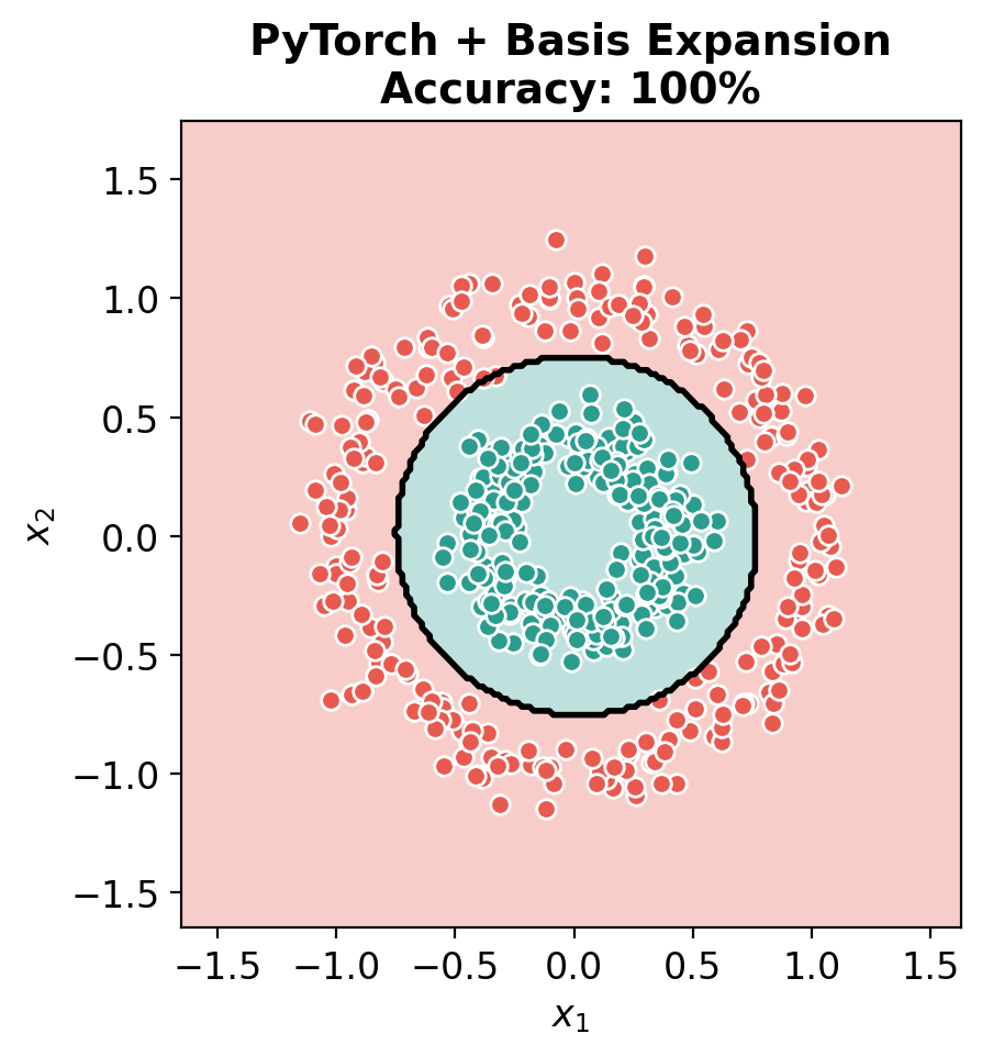
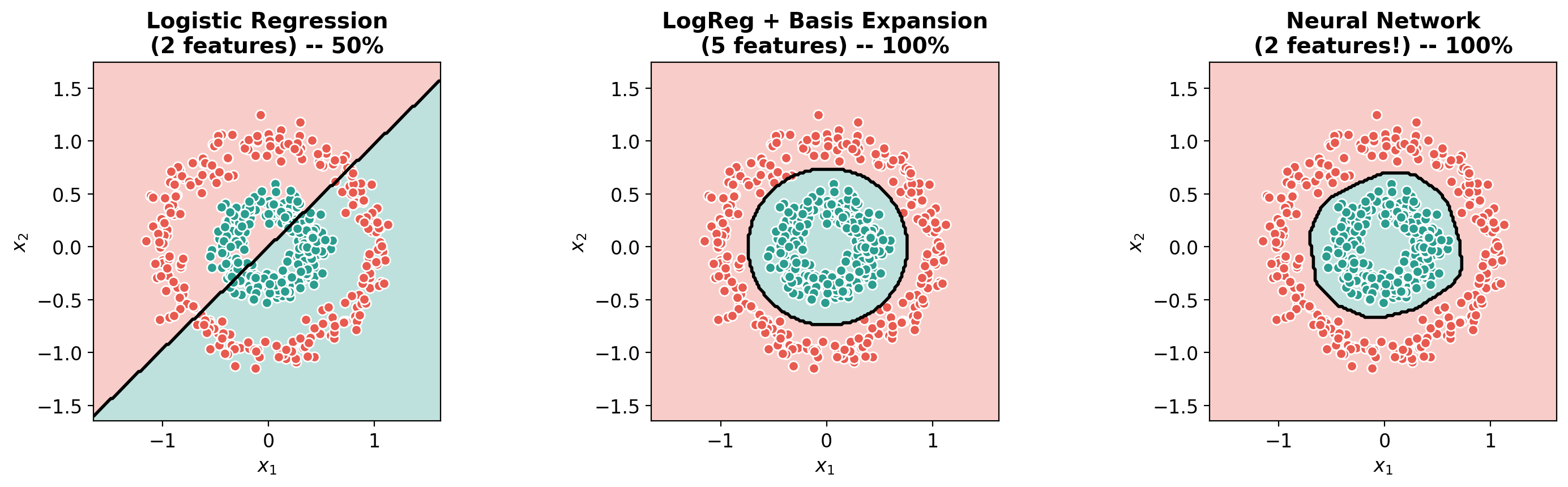
# The big comparison
fig, axes = plt.subplots(1, 3, figsize=(15, 4.5))

plot_decision_boundary(lr_sklearn.predict, X_circles, y_circles,
    f'Logistic Regression\n(2 features) -- {lr_sklearn.score(X_circles, y_circles):.0%}', ax=axes[0])

plot_decision_boundary(predict_poly_sklearn, X_circles, y_circles,
    f'LogReg + Basis Expansion\n(5 features) -- {lr_poly.score(X_poly, y_circles):.0%}', ax=axes[1])

plot_decision_boundary(predict_nn, X_circles, y_circles,
    f'Neural Network\n(2 features!) -- {acc:.0%}', ax=axes[2])

plt.tight_layout()
plt.show()

print('Left:   Linear model on raw features     -- FAILS (can only draw a line)')
print('Middle: Linear model + manual features    -- WORKS (but we had to know which features to add)')
print('Right:  Neural network on raw features    -- WORKS (learns its own features!)')

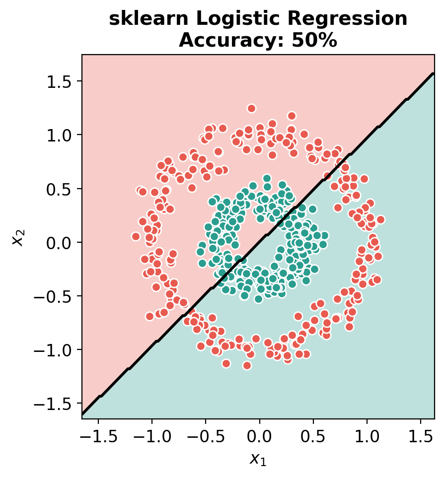
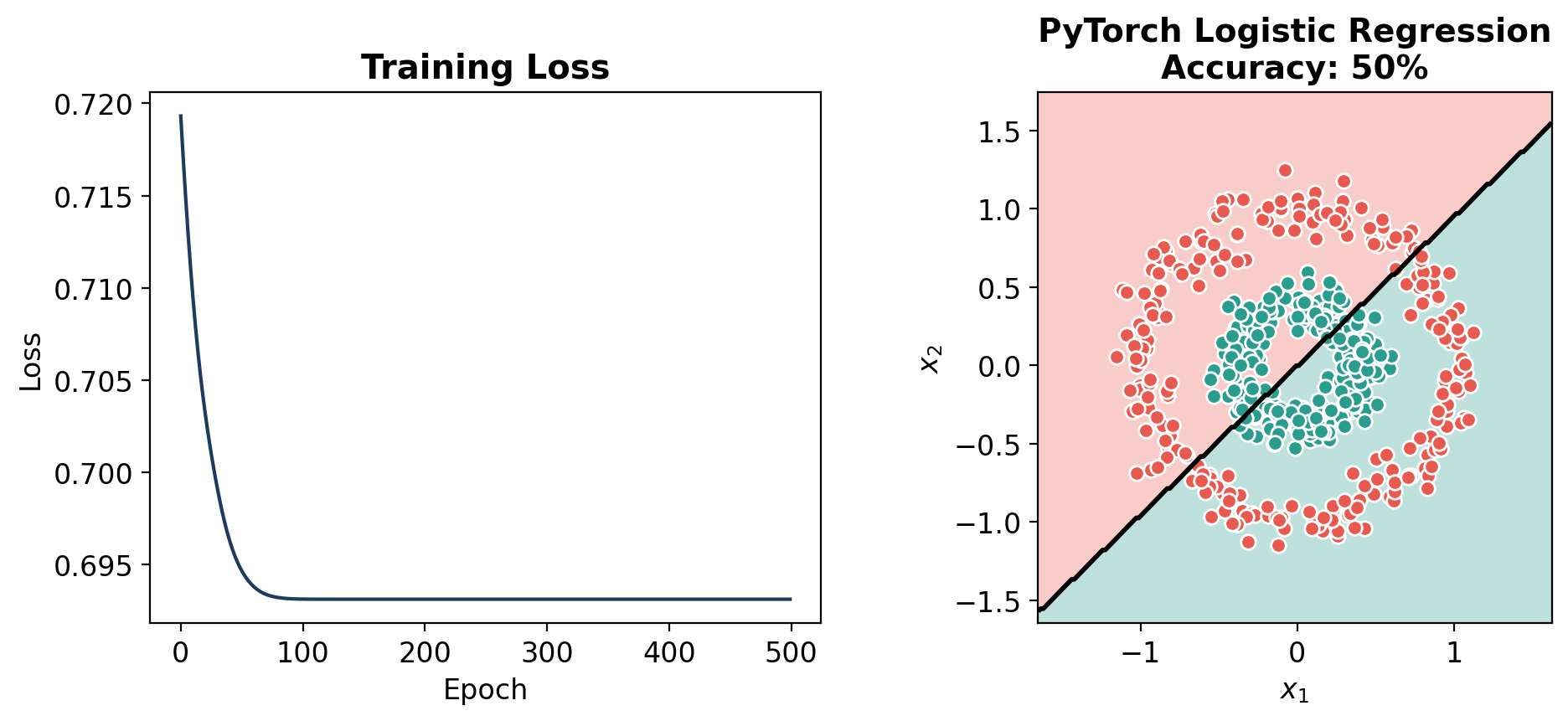
Left:   Linear model on raw features     -- FAILS (can only draw a line)
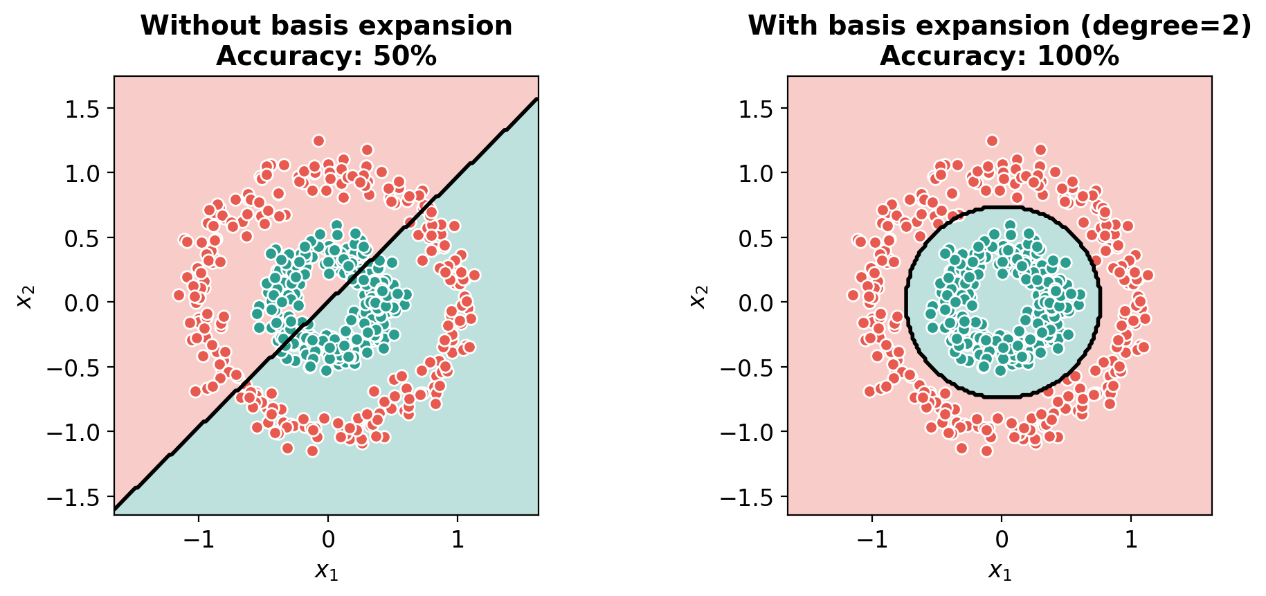
Middle: Linear model + manual features    -- WORKS (but we had to know which features to add)
Right:  Neural network on raw features    -- WORKS (learns its own features!)

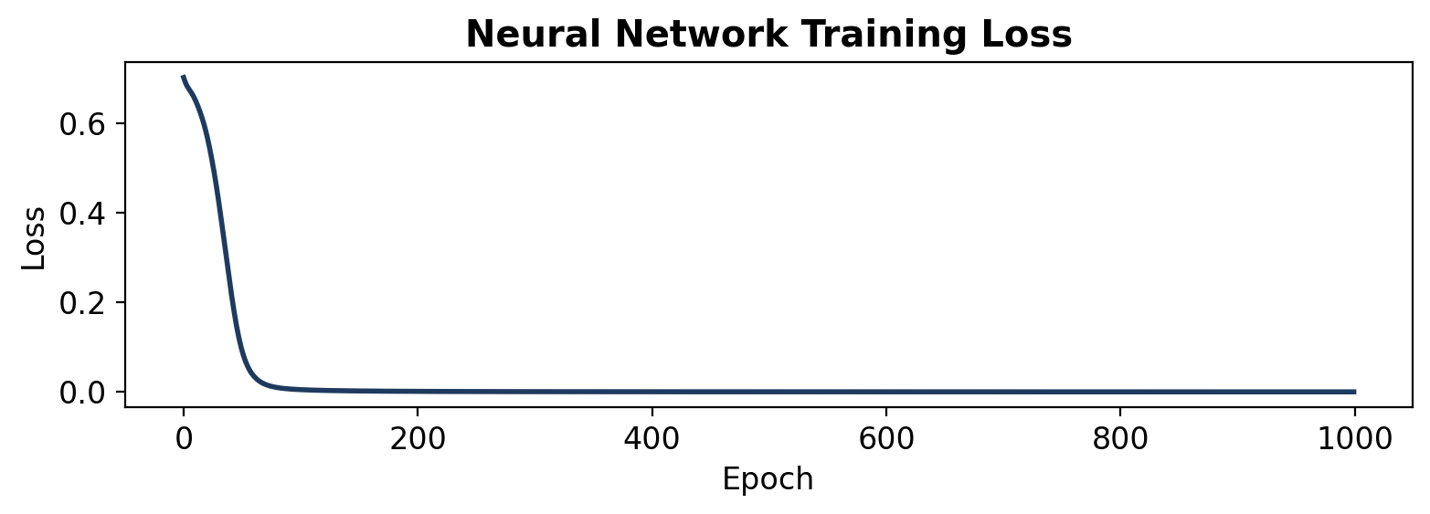
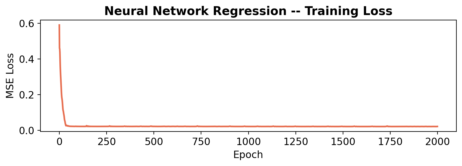
# Training loss curve for the neural network
fig, ax = plt.subplots(figsize=(8, 3))
ax.plot(losses, color='#1e3a5f', linewidth=2)
ax.set_xlabel('Epoch')
ax.set_ylabel('Loss')
ax.set_title('Neural Network Training Loss', fontweight='bold')
plt.tight_layout()
plt.show()

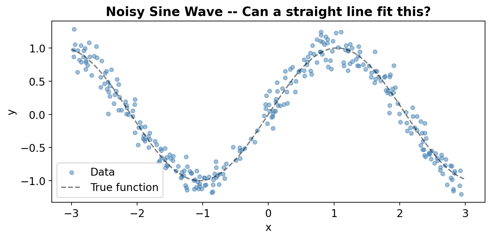
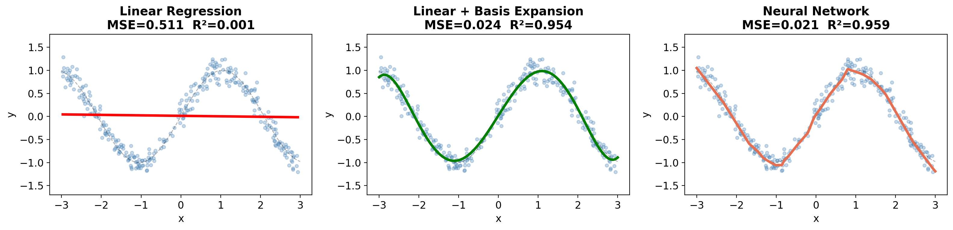
Part 2: Regression – Fitting a Wiggly Curve

Same idea, but for regression. Can a straight line fit a sine wave?

# Generate noisy sine wave data
np.random.seed(42)
n = 300
X_reg = np.sort(np.random.uniform(-3, 3, n))

# True function: a wiggly sine curve
def true_fn(x):
    return np.sin(1.5 * x)

y_reg = true_fn(X_reg) + np.random.normal(0, 0.15, n)

fig, ax = plt.subplots(figsize=(8, 4))
ax.scatter(X_reg, y_reg, alpha=0.5, s=20, color='steelblue', label='Data')
x_dense = np.linspace(-3, 3, 500)
ax.plot(x_dense, true_fn(x_dense), 'k--', alpha=0.5, label='True function')
ax.set_xlabel('x'); ax.set_ylabel('y')
ax.set_title('Noisy Sine Wave -- Can a straight line fit this?', fontweight='bold')
ax.legend()
plt.tight_layout()
plt.show()

Step 1: Linear Regression (sklearn)

from sklearn.metrics import r2_score

# Fit a straight line
lin_sklearn = LinearRegression()
lin_sklearn.fit(X_reg.reshape(-1, 1), y_reg)
y_pred_lin = lin_sklearn.predict(X_reg.reshape(-1, 1))
r2_lin = r2_score(y_reg, y_pred_lin)

fig, ax = plt.subplots(figsize=(8, 4))
ax.scatter(X_reg, y_reg, alpha=0.4, s=20, color='steelblue')
ax.plot(X_reg, y_pred_lin, 'r-', linewidth=3, label=f'Linear fit (R² = {r2_lin:.3f})')
ax.set_xlabel('x'); ax.set_ylabel('y')
ax.set_title('sklearn Linear Regression', fontweight='bold')
ax.legend()
plt.tight_layout()
plt.show()

print(f'R² = {r2_lin:.3f} -- terrible! A line cannot capture the wiggles.')

R² = 0.001 -- terrible! A line cannot capture the wiggles.

Step 2: Linear Regression in PyTorch

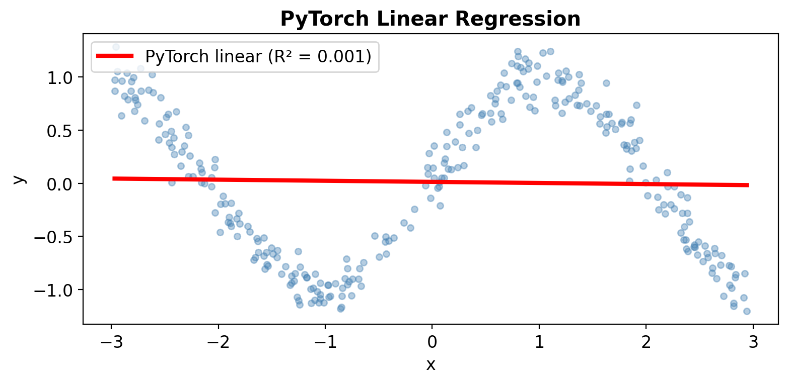
# Same linear regression in PyTorch
X_reg_t = torch.tensor(X_reg, dtype=torch.float32).unsqueeze(1)
y_reg_t = torch.tensor(y_reg, dtype=torch.float32).unsqueeze(1)

torch.manual_seed(42)
lin_torch = nn.Linear(1, 1)
optimizer = optim.Adam(lin_torch.parameters(), lr=0.05)
mse_loss = nn.MSELoss()

for epoch in range(500):
    pred = lin_torch(X_reg_t)
    loss = mse_loss(pred, y_reg_t)
    optimizer.zero_grad()
    loss.backward()
    optimizer.step()

with torch.no_grad():
    y_pred_lin_torch = lin_torch(X_reg_t).numpy()

r2_torch = r2_score(y_reg, y_pred_lin_torch)

fig, ax = plt.subplots(figsize=(8, 4))
ax.scatter(X_reg, y_reg, alpha=0.4, s=20, color='steelblue')
ax.plot(X_reg, y_pred_lin_torch, 'r-', linewidth=3, label=f'PyTorch linear (R² = {r2_torch:.3f})')
ax.set_xlabel('x'); ax.set_ylabel('y')
ax.set_title('PyTorch Linear Regression', fontweight='bold')
ax.legend()
plt.tight_layout()
plt.show()

print(f'Same result: R² = {r2_torch:.3f}')
print('PyTorch linear = sklearn linear. Both can only fit a line.')

Same result: R² = 0.001
PyTorch linear = sklearn linear. Both can only fit a line.

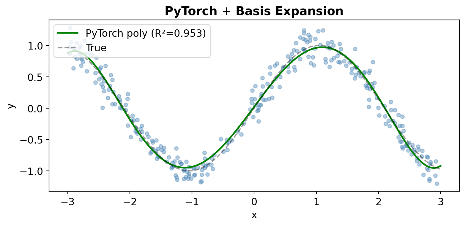
Step 3: Basis Expansion – Adding Polynomial Features

# Basis expansion: add x^2, x^3, x^4, x^5
poly_reg = PolynomialFeatures(degree=5, include_bias=False)
X_reg_poly = poly_reg.fit_transform(X_reg.reshape(-1, 1))

print(f'Original: 1 feature (x)')
print(f'After expansion: {X_reg_poly.shape[1]} features ({" , ".join(poly_reg.get_feature_names_out())})')
print()

# sklearn
lin_poly_sklearn = LinearRegression()
lin_poly_sklearn.fit(X_reg_poly, y_reg)

x_dense_poly = poly_reg.transform(x_dense.reshape(-1, 1))
y_pred_poly = lin_poly_sklearn.predict(x_dense_poly)
r2_poly = r2_score(y_reg, lin_poly_sklearn.predict(X_reg_poly))

fig, axes = plt.subplots(1, 2, figsize=(14, 4))
axes[0].scatter(X_reg, y_reg, alpha=0.4, s=20, color='steelblue')
axes[0].plot(X_reg, y_pred_lin, 'r-', linewidth=2, label=f'Linear (R²={r2_lin:.3f})')
axes[0].set_title('Linear Fit', fontweight='bold')
axes[0].legend(); axes[0].set_xlabel('x'); axes[0].set_ylabel('y')

axes[1].scatter(X_reg, y_reg, alpha=0.4, s=20, color='steelblue')
axes[1].plot(x_dense, y_pred_poly, 'g-', linewidth=2, label=f'Degree 5 (R²={r2_poly:.3f})')
axes[1].plot(x_dense, true_fn(x_dense), 'k--', alpha=0.4, label='True')
axes[1].set_title('Polynomial Basis Expansion (degree=5)', fontweight='bold')
axes[1].legend(); axes[1].set_xlabel('x'); axes[1].set_ylabel('y')

plt.tight_layout()
plt.show()

print(f'With basis expansion: R² = {r2_poly:.3f}')
print('It works! But we had to guess that degree=5 was right.')

Original: 1 feature (x)
After expansion: 5 features (x0 , x0^2 , x0^3 , x0^4 , x0^5)

With basis expansion: R² = 0.954
It works! But we had to guess that degree=5 was right.

# Same in PyTorch
X_reg_poly_t = torch.tensor(X_reg_poly, dtype=torch.float32)

torch.manual_seed(42)
lin_poly_torch = nn.Linear(5, 1)
optimizer = optim.Adam(lin_poly_torch.parameters(), lr=0.05)

for epoch in range(1000):
    pred = lin_poly_torch(X_reg_poly_t)
    loss = mse_loss(pred, y_reg_t)
    optimizer.zero_grad()
    loss.backward()
    optimizer.step()

with torch.no_grad():
    x_dense_t = torch.tensor(x_dense_poly, dtype=torch.float32)
    y_pred_poly_torch = lin_poly_torch(x_dense_t).numpy()
    r2_pt = r2_score(y_reg, lin_poly_torch(X_reg_poly_t).numpy())

fig, ax = plt.subplots(figsize=(8, 4))
ax.scatter(X_reg, y_reg, alpha=0.4, s=20, color='steelblue')
ax.plot(x_dense, y_pred_poly_torch, 'g-', linewidth=2, label=f'PyTorch poly (R²={r2_pt:.3f})')
ax.plot(x_dense, true_fn(x_dense), 'k--', alpha=0.4, label='True')
ax.set_title('PyTorch + Basis Expansion', fontweight='bold')
ax.legend(); ax.set_xlabel('x'); ax.set_ylabel('y')
plt.tight_layout()
plt.show()

Step 4: Neural Network – Learns the Curve Automatically

# Neural network on original 1 feature -- NO basis expansion
torch.manual_seed(42)
nn_reg = nn.Sequential(
    nn.Linear(1, 32),
    nn.ReLU(),
    nn.Linear(32, 32),
    nn.ReLU(),
    nn.Linear(32, 1)
)

optimizer = optim.Adam(nn_reg.parameters(), lr=0.01)

losses = []
for epoch in range(2000):
    pred = nn_reg(X_reg_t)
    loss = mse_loss(pred, y_reg_t)
    optimizer.zero_grad()
    loss.backward()
    optimizer.step()
    losses.append(loss.item())

with torch.no_grad():
    x_dense_t1 = torch.tensor(x_dense, dtype=torch.float32).unsqueeze(1)
    y_pred_nn = nn_reg(x_dense_t1).numpy()
    r2_nn = r2_score(y_reg, nn_reg(X_reg_t).numpy())

print(f'Neural Network R² = {r2_nn:.3f}')

Neural Network R² = 0.959

from sklearn.metrics import mean_squared_error

# Compute MSE for all models
with torch.no_grad():
    mse_lin = mean_squared_error(y_reg, y_pred_lin)
    mse_poly = mean_squared_error(y_reg, lin_poly_sklearn.predict(X_reg_poly))
    mse_nn = mean_squared_error(y_reg, nn_reg(X_reg_t).numpy())

# The big regression comparison
fig, axes = plt.subplots(1, 3, figsize=(16, 4))

for ax in axes:
    ax.scatter(X_reg, y_reg, alpha=0.3, s=15, color='steelblue')
    ax.plot(x_dense, true_fn(x_dense), 'k--', alpha=0.3, linewidth=1)
    ax.set_xlabel('x'); ax.set_ylabel('y')
    ax.set_ylim(y_reg.min() - 0.5, y_reg.max() + 0.5)

axes[0].plot(X_reg, y_pred_lin, 'r-', linewidth=3)
axes[0].set_title(f'Linear Regression\nMSE={mse_lin:.3f}  R²={r2_lin:.3f}', fontweight='bold')

axes[1].plot(x_dense, y_pred_poly, 'g-', linewidth=3)
axes[1].set_title(f'Linear + Basis Expansion\nMSE={mse_poly:.3f}  R²={r2_poly:.3f}', fontweight='bold')

axes[2].plot(x_dense, y_pred_nn.ravel(), '#e76f51', linewidth=3)
axes[2].set_title(f'Neural Network\nMSE={mse_nn:.3f}  R²={r2_nn:.3f}', fontweight='bold')

plt.tight_layout()
plt.show()

print(f'{"Model":<30} {"MSE":>8} {"R²":>8}')
print('-' * 48)
print(f'{"Linear (1 feature)":<30} {mse_lin:>8.4f} {r2_lin:>8.3f}')
print(f'{"Linear + poly features (5)":<30} {mse_poly:>8.4f} {r2_poly:>8.3f}')
print(f'{"Neural network (1 feature!)":<30} {mse_nn:>8.4f} {r2_nn:>8.3f}')

Model                               MSE       R²
------------------------------------------------
Linear (1 feature)               0.5111    0.001
Linear + poly features (5)       0.0238    0.954
Neural network (1 feature!)      0.0211    0.959

fig, ax = plt.subplots(figsize=(8, 3))
ax.plot(losses, color='#e76f51', linewidth=2)
ax.set_xlabel('Epoch')
ax.set_ylabel('MSE Loss')
ax.set_title('Neural Network Regression -- Training Loss', fontweight='bold')
plt.tight_layout()
plt.show()

Interim Takeaway

Approach	Features	Works?	Problem
Linear model	Raw \((x_1, x_2)\)	No	Can only draw straight lines
Linear model + basis expansion	Manual \((x_1, x_2, x_1^2, x_2^2, ...)\)	Yes	You must know which features to add
Neural network	Raw \((x_1, x_2)\)	Yes	Learns its own features automatically!

But those were easy examples. What about harder data where you can’t guess the right features?

Part 3: When Feature Engineering Breaks Down – Spirals

Concentric circles were “easy” – we knew the boundary was \(x_1^2 + x_2^2 = r^2\).

What about data where you have no idea what features to add?

# Generate spiral data -- much harder than circles!
np.random.seed(42)
n_per_class = 300

theta0 = np.linspace(0, 3 * np.pi, n_per_class) + np.random.normal(0, 0.15, n_per_class)
r0 = theta0 / (3 * np.pi)
x0 = np.c_[r0 * np.cos(theta0), r0 * np.sin(theta0)]

theta1 = np.linspace(0, 3 * np.pi, n_per_class) + np.random.normal(0, 0.15, n_per_class)
r1 = theta1 / (3 * np.pi)
x1 = np.c_[r1 * np.cos(theta1 + np.pi), r1 * np.sin(theta1 + np.pi)]

X_spiral = np.vstack([x0, x1])
y_spiral = np.array([0] * n_per_class + [1] * n_per_class)

fig, ax = plt.subplots(figsize=(6, 6))
ax.scatter(X_spiral[y_spiral == 0, 0], X_spiral[y_spiral == 0, 1], c=C0, s=15, alpha=0.7, label='Class 0')
ax.scatter(X_spiral[y_spiral == 1, 0], X_spiral[y_spiral == 1, 1], c=C1, s=15, alpha=0.7, label='Class 1')
ax.set_title('Two Spirals -- Try drawing ANY simple boundary!', fontsize=14, fontweight='bold')
ax.set_xlabel('$x_1$'); ax.set_ylabel('$x_2$')
ax.legend()
ax.set_aspect('equal')
plt.tight_layout()
plt.show()

print('No polynomial, no simple formula can separate these spirals.')
print('You would need to engineer very exotic features (polar coords, angles, etc.)')

No polynomial, no simple formula can separate these spirals.
You would need to engineer very exotic features (polar coords, angles, etc.)

# Try everything we know: logistic regression, polynomial basis expansion, neural network
from sklearn.pipeline import make_pipeline

# 1. Logistic regression (linear)
lr_spiral = LogisticRegression()
lr_spiral.fit(X_spiral, y_spiral)

# 2. Polynomial basis expansion -- even degree 6 won't cut it
poly_spiral = PolynomialFeatures(degree=6, include_bias=False)
X_spiral_poly = poly_spiral.fit_transform(X_spiral)
lr_spiral_poly = LogisticRegression(max_iter=5000, C=10)
lr_spiral_poly.fit(X_spiral_poly, y_spiral)

print(f'Polynomial features: {X_spiral_poly.shape[1]} features from degree-6 expansion!')

def predict_spiral_poly(X_np):
    return lr_spiral_poly.predict(poly_spiral.transform(X_np))

# 3. Neural network
X_spiral_t = torch.tensor(X_spiral, dtype=torch.float32)
y_spiral_t = torch.tensor(y_spiral, dtype=torch.float32).unsqueeze(1)

torch.manual_seed(42)
nn_spiral = nn.Sequential(
    nn.Linear(2, 64),
    nn.ReLU(),
    nn.Linear(64, 64),
    nn.ReLU(),
    nn.Linear(64, 32),
    nn.ReLU(),
    nn.Linear(32, 1),
    nn.Sigmoid()
)

optimizer = optim.Adam(nn_spiral.parameters(), lr=0.005)
loss_fn = nn.BCELoss()

for epoch in range(3000):
    pred = nn_spiral(X_spiral_t)
    loss = loss_fn(pred, y_spiral_t)
    optimizer.zero_grad()
    loss.backward()
    optimizer.step()

def predict_nn_spiral(X_np):
    with torch.no_grad():
        probs = nn_spiral(torch.tensor(X_np, dtype=torch.float32))
        return (probs.numpy() > 0.5).astype(int).ravel()

acc_lin = lr_spiral.score(X_spiral, y_spiral)
acc_poly = lr_spiral_poly.score(X_spiral_poly, y_spiral)
acc_nn = (predict_nn_spiral(X_spiral) == y_spiral).mean()

print(f'\nLinear:                 {acc_lin:.0%}')
print(f'Poly (degree 6, {X_spiral_poly.shape[1]} features): {acc_poly:.0%}')
print(f'Neural Network (2 raw features): {acc_nn:.0%}')

Polynomial features: 27 features from degree-6 expansion!

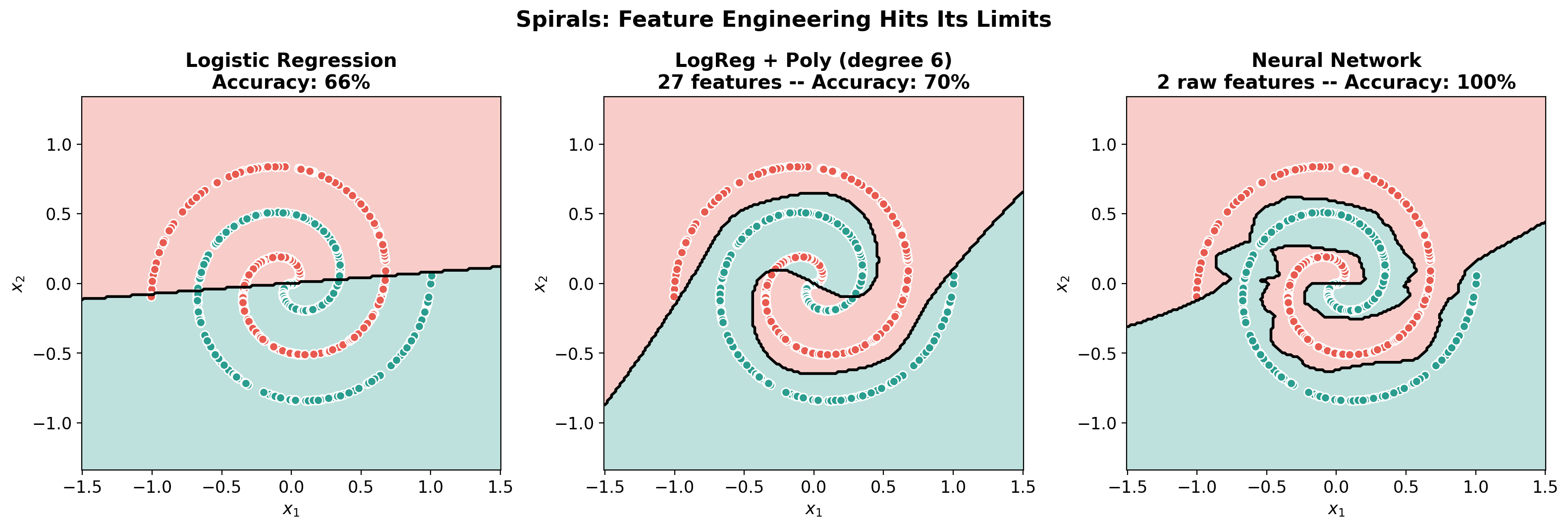
Linear:                 66%
Poly (degree 6, 27 features): 70%
Neural Network (2 raw features): 100%

# Decision boundary comparison
fig, axes = plt.subplots(1, 3, figsize=(16, 5))

plot_decision_boundary(lr_spiral.predict, X_spiral, y_spiral,
    f'Logistic Regression\nAccuracy: {acc_lin:.0%}', ax=axes[0])

plot_decision_boundary(predict_spiral_poly, X_spiral, y_spiral,
    f'LogReg + Poly (degree 6)\n{X_spiral_poly.shape[1]} features -- Accuracy: {acc_poly:.0%}', ax=axes[1])

plot_decision_boundary(predict_nn_spiral, X_spiral, y_spiral,
    f'Neural Network\n2 raw features -- Accuracy: {acc_nn:.0%}', ax=axes[2])

plt.suptitle('Spirals: Feature Engineering Hits Its Limits', fontsize=16, fontweight='bold', y=1.02)
plt.tight_layout()
plt.show()

print('Even with 27 polynomial features, logistic regression struggles.')
print('The neural network learns the spiral boundary from just x1 and x2!')
print('\nThis is the real power: NNs handle patterns that no human would think to engineer.')

Even with 27 polynomial features, logistic regression struggles.
The neural network learns the spiral boundary from just x1 and x2!

This is the real power: NNs handle patterns that no human would think to engineer.

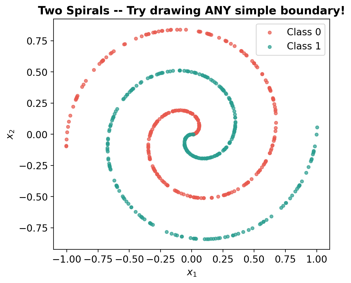
Part 4: Images – Where Feature Engineering Really Falls Apart

For circles and spirals, a clever person might guess polar coordinates or high-degree polynomials.

But what about images? Before deep learning, computer vision relied on: - Pixel intensity histograms - HOG (Histogram of Oriented Gradients) – edge directions - SIFT/SURF – local keypoints - Manually designed for each task!

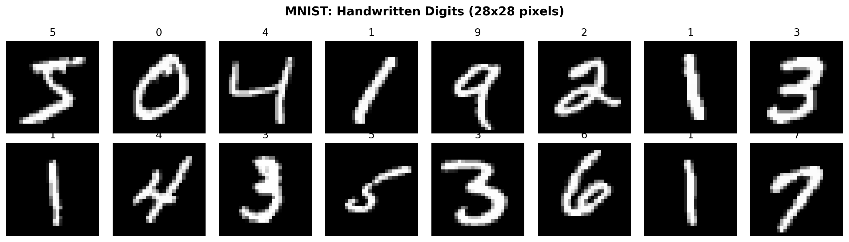
Let’s see this on MNIST digit classification.

# Load MNIST
from torchvision import datasets, transforms
from sklearn.metrics import accuracy_score

mnist_train = datasets.MNIST('./data', train=True, download=True)
mnist_test = datasets.MNIST('./data', train=False, download=True)

# Convert to numpy
X_train_img = mnist_train.data.numpy()  # (60000, 28, 28)
y_train_img = mnist_train.targets.numpy()
X_test_img = mnist_test.data.numpy()
y_test_img = mnist_test.targets.numpy()

# Show some samples
fig, axes = plt.subplots(2, 8, figsize=(14, 4))
for i, ax in enumerate(axes.ravel()):
    ax.imshow(X_train_img[i], cmap='gray')
    ax.set_title(f'{y_train_img[i]}', fontsize=12)
    ax.axis('off')
plt.suptitle('MNIST: Handwritten Digits (28x28 pixels)', fontsize=14, fontweight='bold')
plt.tight_layout()
plt.show()

print(f'Training set: {X_train_img.shape[0]} images, {X_train_img.shape[1]}x{X_train_img.shape[2]} pixels')
print(f'Test set:     {X_test_img.shape[0]} images')
print(f'Task: classify each image into one of 10 digits (0-9)')

Training set: 60000 images, 28x28 pixels
Test set:     10000 images
Task: classify each image into one of 10 digits (0-9)

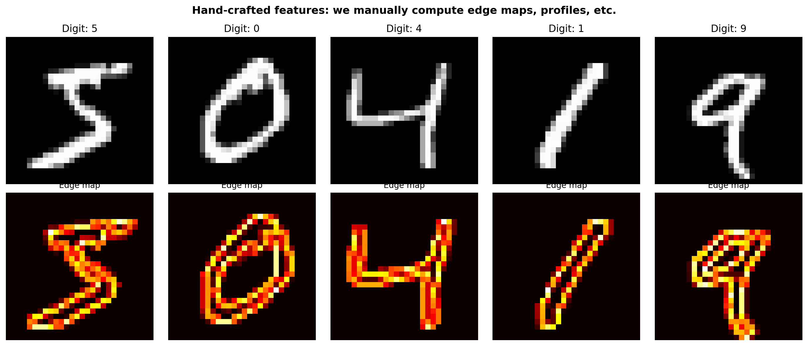
Approach 1: Hand-Crafted Features + Logistic Regression

The “old way” – before deep learning, you’d manually design features: - Raw pixels flattened into a vector (784 numbers) - Intensity features: mean brightness, how much ink, symmetry - HOG features: captures edge directions (the standard pre-deep-learning feature)

def extract_handcrafted_features(images):
    """Extract hand-designed features from digit images.
    This is what engineers did BEFORE deep learning."""
    features = []
    for img in images:
        img_f = img.astype(np.float32) / 255.0
        
        # 1. Basic intensity features
        mean_intensity = img_f.mean()
        std_intensity = img_f.std()
        ink_ratio = (img_f > 0.3).mean()  # fraction of "ink" pixels
        
        # 2. Spatial features -- where is the ink?
        top_half = img_f[:14, :].mean()
        bottom_half = img_f[14:, :].mean()
        left_half = img_f[:, :14].mean()
        right_half = img_f[:, 14:].mean()
        vertical_symmetry = np.abs(top_half - bottom_half)
        horizontal_symmetry = np.abs(left_half - right_half)
        
        # 3. Quadrant features
        q1 = img_f[:14, :14].mean()
        q2 = img_f[:14, 14:].mean()
        q3 = img_f[14:, :14].mean()
        q4 = img_f[14:, 14:].mean()
        
        # 4. Simple edge features (horizontal & vertical gradients)
        grad_h = np.abs(np.diff(img_f, axis=1)).mean()
        grad_v = np.abs(np.diff(img_f, axis=0)).mean()
        
        # 5. Profile features -- project onto axes
        row_profile = img_f.mean(axis=1)  # 28 values
        col_profile = img_f.mean(axis=0)  # 28 values
        
        feat = [mean_intensity, std_intensity, ink_ratio,
                top_half, bottom_half, left_half, right_half,
                vertical_symmetry, horizontal_symmetry,
                q1, q2, q3, q4, grad_h, grad_v]
        feat.extend(row_profile)
        feat.extend(col_profile)
        features.append(feat)
    
    return np.array(features)

# Extract features
print('Extracting hand-crafted features...')
X_train_feat = extract_handcrafted_features(X_train_img)
X_test_feat = extract_handcrafted_features(X_test_img)
print(f'Hand-crafted features per image: {X_train_feat.shape[1]}')
print(f'  - 15 engineered features (intensity, symmetry, gradients, quadrants)')
print(f'  - 28 row profile + 28 column profile')

# Visualize what HOG-like features look like
fig, axes = plt.subplots(2, 5, figsize=(14, 6))
for i in range(5):
    img = X_train_img[i].astype(np.float32) / 255.0
    axes[0, i].imshow(img, cmap='gray')
    axes[0, i].set_title(f'Digit: {y_train_img[i]}', fontsize=12)
    axes[0, i].axis('off')
    
    # Show gradient magnitude (edge map)
    gx = np.abs(np.diff(img, axis=1, prepend=0))
    gy = np.abs(np.diff(img, axis=0, prepend=0))
    edges = np.sqrt(gx**2 + gy**2)
    axes[1, i].imshow(edges, cmap='hot')
    axes[1, i].set_title('Edge map', fontsize=10)
    axes[1, i].axis('off')

axes[0, 0].set_ylabel('Original', fontsize=12)
axes[1, 0].set_ylabel('Edges', fontsize=12)
plt.suptitle('Hand-crafted features: we manually compute edge maps, profiles, etc.', 
             fontsize=13, fontweight='bold')
plt.tight_layout()
plt.show()

Extracting hand-crafted features...
Hand-crafted features per image: 71
  - 15 engineered features (intensity, symmetry, gradients, quadrants)
  - 28 row profile + 28 column profile

# --- Model 1: Logistic Regression on raw pixels ---
X_train_flat = X_train_img.reshape(-1, 784).astype(np.float32) / 255.0
X_test_flat = X_test_img.reshape(-1, 784).astype(np.float32) / 255.0

print('Training logistic regression on raw pixels (784 features)...')
lr_pixels = LogisticRegression(max_iter=1000, solver='lbfgs')
lr_pixels.fit(X_train_flat, y_train_img)
acc_pixels = accuracy_score(y_test_img, lr_pixels.predict(X_test_flat))
print(f'  Test accuracy: {acc_pixels:.1%}')

# --- Model 2: Logistic Regression on hand-crafted features ---
print(f'\nTraining logistic regression on hand-crafted features ({X_train_feat.shape[1]} features)...')
lr_feat = LogisticRegression(max_iter=1000, solver='lbfgs')
lr_feat.fit(X_train_feat, y_train_img)
acc_feat = accuracy_score(y_test_img, lr_feat.predict(X_test_feat))
print(f'  Test accuracy: {acc_feat:.1%}')

Training logistic regression on raw pixels (784 features)...
  Test accuracy: 92.6%

Training logistic regression on hand-crafted features (71 features)...
  Test accuracy: 84.5%

Approach 2: Simple CNN – Let the Network Learn Its Own Features

Instead of us designing edge detectors, the CNN learns what patterns matter.

A convolution layer is like a tiny sliding window that learns to detect edges, curves, loops – whatever helps classify the digit.

# Simple CNN -- just 3 layers, nothing fancy
class SimpleCNN(nn.Module):
    def __init__(self):
        super().__init__()
        self.features = nn.Sequential(
            nn.Conv2d(1, 16, 3, padding=1),  # 28x28 -> 28x28, 16 filters
            nn.ReLU(),
            nn.MaxPool2d(2),                  # 28x28 -> 14x14
            nn.Conv2d(16, 32, 3, padding=1), # 14x14 -> 14x14, 32 filters
            nn.ReLU(),
            nn.MaxPool2d(2),                  # 14x14 -> 7x7
        )
        self.classifier = nn.Sequential(
            nn.Flatten(),
            nn.Linear(32 * 7 * 7, 64),
            nn.ReLU(),
            nn.Linear(64, 10)
        )
    
    def forward(self, x):
        x = self.features(x)
        x = self.classifier(x)
        return x

torch.manual_seed(42)
cnn = SimpleCNN()
n_params = sum(p.numel() for p in cnn.parameters())
print(f'CNN architecture:')
print(cnn)
print(f'\nTotal parameters: {n_params:,}')

CNN architecture:
SimpleCNN(
  (features): Sequential(
    (0): Conv2d(1, 16, kernel_size=(3, 3), stride=(1, 1), padding=(1, 1))
    (1): ReLU()
    (2): MaxPool2d(kernel_size=2, stride=2, padding=0, dilation=1, ceil_mode=False)
    (3): Conv2d(16, 32, kernel_size=(3, 3), stride=(1, 1), padding=(1, 1))
    (4): ReLU()
    (5): MaxPool2d(kernel_size=2, stride=2, padding=0, dilation=1, ceil_mode=False)
  )
  (classifier): Sequential(
    (0): Flatten(start_dim=1, end_dim=-1)
    (1): Linear(in_features=1568, out_features=64, bias=True)
    (2): ReLU()
    (3): Linear(in_features=64, out_features=10, bias=True)
  )
)

Total parameters: 105,866

# Train the CNN
# Prepare data as tensors -- images need shape (N, 1, 28, 28)
X_train_cnn = torch.tensor(X_train_img, dtype=torch.float32).unsqueeze(1) / 255.0
y_train_cnn = torch.tensor(y_train_img, dtype=torch.long)
X_test_cnn = torch.tensor(X_test_img, dtype=torch.float32).unsqueeze(1) / 255.0
y_test_cnn = torch.tensor(y_test_img, dtype=torch.long)

optimizer = optim.Adam(cnn.parameters(), lr=0.001)
loss_fn_ce = nn.CrossEntropyLoss()

# Train for 3 epochs using mini-batches
batch_size = 256
losses_cnn = []

for epoch in range(3):
    epoch_loss = 0
    n_batches = 0
    # Shuffle
    perm = torch.randperm(len(X_train_cnn))
    
    for i in range(0, len(X_train_cnn), batch_size):
        idx = perm[i:i+batch_size]
        X_batch = X_train_cnn[idx]
        y_batch = y_train_cnn[idx]
        
        pred = cnn(X_batch)
        loss = loss_fn_ce(pred, y_batch)
        
        optimizer.zero_grad()
        loss.backward()
        optimizer.step()
        
        epoch_loss += loss.item()
        n_batches += 1
        losses_cnn.append(loss.item())
    
    # Evaluate
    with torch.no_grad():
        # Test in batches to avoid memory issues
        correct = 0
        for i in range(0, len(X_test_cnn), 1000):
            preds = cnn(X_test_cnn[i:i+1000]).argmax(dim=1)
            correct += (preds == y_test_cnn[i:i+1000]).sum().item()
        acc_cnn = correct / len(y_test_cnn)
    
    print(f'Epoch {epoch+1}/3 -- Loss: {epoch_loss/n_batches:.4f} -- Test Accuracy: {acc_cnn:.1%}')

print(f'\nFinal CNN test accuracy: {acc_cnn:.1%}')

Epoch 1/3 -- Loss: 0.4998 -- Test Accuracy: 94.6%
Epoch 2/3 -- Loss: 0.1225 -- Test Accuracy: 97.5%
Epoch 3/3 -- Loss: 0.0792 -- Test Accuracy: 98.0%

Final CNN test accuracy: 98.0%

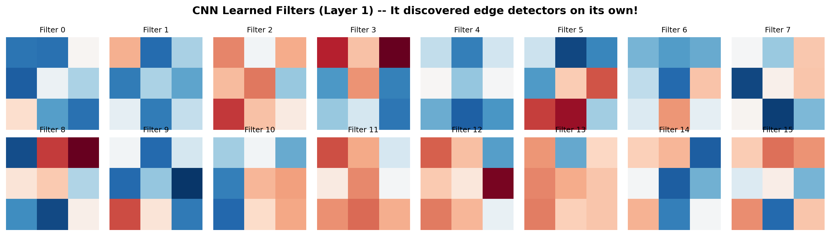
# What did the CNN learn? Visualize the first-layer filters
fig, axes = plt.subplots(2, 8, figsize=(14, 4))
filters = cnn.features[0].weight.data.numpy()  # (16, 1, 3, 3)
for i, ax in enumerate(axes.ravel()):
    ax.imshow(filters[i, 0], cmap='RdBu', vmin=-0.5, vmax=0.5)
    ax.set_title(f'Filter {i}', fontsize=9)
    ax.axis('off')
plt.suptitle('CNN Learned Filters (Layer 1) -- It discovered edge detectors on its own!', 
             fontsize=13, fontweight='bold')
plt.tight_layout()
plt.show()

print('These filters detect edges, corners, and gradients.')
print('We never told the CNN to look for edges -- it figured it out from the data!')

These filters detect edges, corners, and gradients.
We never told the CNN to look for edges -- it figured it out from the data!

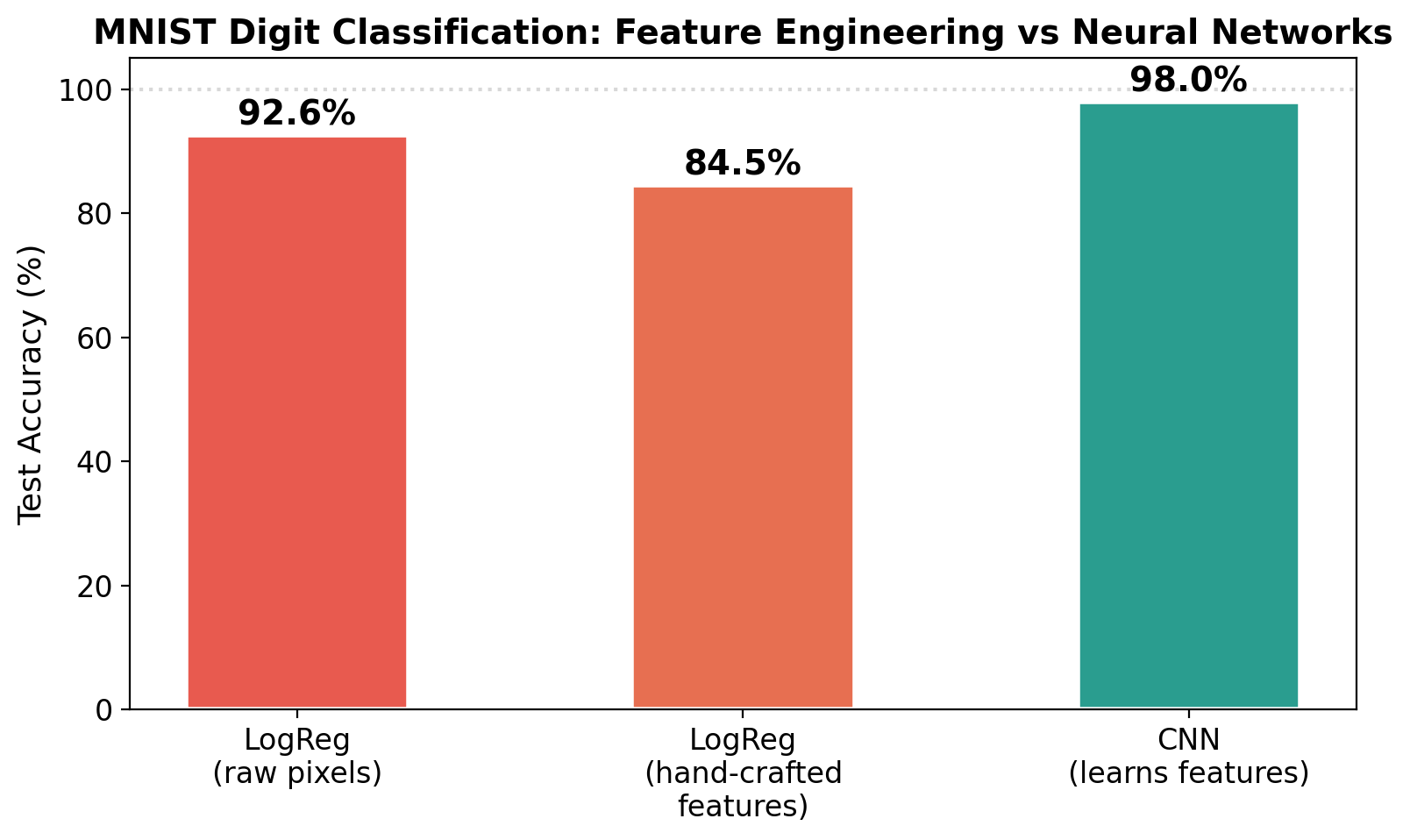
# The big comparison -- bar chart
models = ['LogReg\n(raw pixels)', 'LogReg\n(hand-crafted\nfeatures)', 'CNN\n(learns features)']
accs = [acc_pixels, acc_feat, acc_cnn]
colors = ['#e85a4f', '#e76f51', '#2a9d8f']

fig, ax = plt.subplots(figsize=(8, 5))
bars = ax.bar(models, [a * 100 for a in accs], color=colors, edgecolor='white', linewidth=2, width=0.5)

for bar, acc in zip(bars, accs):
    ax.text(bar.get_x() + bar.get_width()/2, bar.get_height() + 0.5,
            f'{acc:.1%}', ha='center', va='bottom', fontsize=14, fontweight='bold')

ax.set_ylabel('Test Accuracy (%)', fontsize=13)
ax.set_title('MNIST Digit Classification: Feature Engineering vs Neural Networks', 
             fontsize=14, fontweight='bold')
ax.set_ylim(0, 105)
ax.axhline(y=100, color='gray', linestyle=':', alpha=0.3)
plt.tight_layout()
plt.show()

print(f'Logistic Regression (784 raw pixels):        {acc_pixels:.1%}')
print(f'Logistic Regression ({X_train_feat.shape[1]} hand-crafted features): {acc_feat:.1%}')
print(f'Simple CNN (learns its own features):        {acc_cnn:.1%}')
print()
print('The CNN beats both -- and we spent ZERO time designing features!')

Logistic Regression (784 raw pixels):        92.6%
Logistic Regression (71 hand-crafted features): 84.5%
Simple CNN (learns its own features):        98.0%

The CNN beats both -- and we spent ZERO time designing features!

The Full Picture

Problem	Feature Engineering	Neural Network
Circles (2D)	Polynomial degree 2 – works (easy to guess)	MLP – works
Spirals (2D)	Polynomial degree 6 – struggles	MLP – works
Sine wave (1D)	Polynomial degree 5 – works (if you guess right)	MLP – works
Digits (images)	Intensity + edges + profiles – OK (~91%)	CNN – great (~99%)

The pattern: - Simple problems: feature engineering can match neural networks - Complex problems: feature engineering breaks down; neural networks scale - Images, audio, text: forget manual features – neural networks dominate

This is the paradigm shift:

Old way: Human designs features → simple model

New way: Raw data → neural network learns everything

The hidden layers of a neural network are the feature engineering – learned from data instead of designed by hand.