The Perceptron

The simplest neural network: one neuron.

We’ll train it the same way we train big networks – forward pass, compute loss, update weights.

  1. What is a perceptron?
  2. Train it to learn AND, OR, NOT, NAND
  3. Watch it fail on XOR
  4. Visualize decision surfaces
import numpy as np
import matplotlib.pyplot as plt
import torch
import torch.nn as nn
import torch.optim as optim
import warnings
warnings.filterwarnings('ignore')

plt.rcParams['figure.figsize'] = (10, 4)
plt.rcParams['font.size'] = 12

C0, C1 = '#e85a4f', '#2a9d8f'
print('Ready!')
%config InlineBackend.figure_format = 'retina'
Ready!

What is a Perceptron?

\[y = \text{activation}(w_1 x_1 + w_2 x_2 + b)\]

  • Takes inputs \(x_1, x_2\)
  • Multiplies by weights \(w_1, w_2\)
  • Adds bias \(b\)
  • Passes through an activation function

Classic vs Modern Perceptron

The original perceptron (Rosenblatt, 1958) used a step function:

\[\text{step}(z) = \begin{cases} 1 & \text{if } z > 0 \\ 0 & \text{otherwise} \end{cases}\]

But step functions have zero gradient – we can’t use gradient descent to train them!

Modern approach: use sigmoid \(\sigma(z) = \frac{1}{1+e^{-z}}\) – smooth version of step, trainable with gradient descent.

Either way, one neuron = one straight decision boundary.

# Visualize: step vs sigmoid
z = np.linspace(-5, 5, 200)
step = (z > 0).astype(float)
sigmoid = 1 / (1 + np.exp(-z))

fig, axes = plt.subplots(1, 2, figsize=(12, 4))
axes[0].plot(z, step, 'r-', linewidth=3)
axes[0].set_title('Step Function (classic perceptron)', fontweight='bold')
axes[0].set_xlabel('z'); axes[0].set_ylabel('output')
axes[0].axhline(y=0.5, color='gray', linestyle=':', alpha=0.5)
axes[0].axvline(x=0, color='gray', linestyle=':', alpha=0.5)
axes[0].text(1, 0.3, 'Not differentiable!\nCan\'t use gradient descent', fontsize=10, color='red')

axes[1].plot(z, sigmoid, 'b-', linewidth=3)
axes[1].set_title('Sigmoid (modern, trainable)', fontweight='bold')
axes[1].set_xlabel('z'); axes[1].set_ylabel('output')
axes[1].axhline(y=0.5, color='gray', linestyle=':', alpha=0.5)
axes[1].axvline(x=0, color='gray', linestyle=':', alpha=0.5)
axes[1].text(1, 0.3, 'Smooth!\nGradient descent works', fontsize=10, color='blue')

plt.tight_layout()
plt.show()

print('We use sigmoid so we can train with gradient descent.')
print('The decision boundary (where output = 0.5) is the same: a straight line.')

We use sigmoid so we can train with gradient descent.
The decision boundary (where output = 0.5) is the same: a straight line.
class Perceptron(nn.Module):
    """A single neuron with sigmoid activation."""
    def __init__(self):
        super().__init__()
        self.linear = nn.Linear(2, 1)
        self.sigmoid = nn.Sigmoid()
    
    def forward(self, x):
        return self.sigmoid(self.linear(x))

print('Perceptron = Linear(2, 1) + Sigmoid')
p = Perceptron()
print(f'Parameters: w1, w2, b = {p.linear.weight.data.numpy().ravel()}, {p.linear.bias.data.item():.4f}')
print(f'Total parameters: {sum(p.numel() for p in p.parameters())} (2 weights + 1 bias)')
Perceptron = Linear(2, 1) + Sigmoid
Parameters: w1, w2, b = [-0.655962   -0.44515052], -0.1790
Total parameters: 3 (2 weights + 1 bias)

Training a Perceptron on Logic Gates

Logic gates are the simplest classification problems: 4 data points, 2 classes.

# All logic gate datasets
X_gate = torch.tensor([[0, 0], [0, 1], [1, 0], [1, 1]], dtype=torch.float32)

gates = {
    'AND':  torch.tensor([[0], [0], [0], [1]], dtype=torch.float32),
    'OR':   torch.tensor([[0], [1], [1], [1]], dtype=torch.float32),
    'NAND': torch.tensor([[1], [1], [1], [0]], dtype=torch.float32),
    'XOR':  torch.tensor([[0], [1], [1], [0]], dtype=torch.float32),
}

# Show truth tables
print(f'{"x1":>3} {"x2":>3}  |  {"AND":>4} {"OR":>4} {"NAND":>5} {"XOR":>4}')
print('-' * 42)
for i in range(4):
    x1, x2 = int(X_gate[i, 0]), int(X_gate[i, 1])
    vals = [int(gates[g][i].item()) for g in ['AND', 'OR', 'NAND', 'XOR']]
    print(f'{x1:>3} {x2:>3}  |  {vals[0]:>4} {vals[1]:>4} {vals[2]:>5} {vals[3]:>4}')
 x1  x2  |   AND   OR  NAND  XOR
------------------------------------------
  0   0  |     0    0     1    0
  0   1  |     0    1     1    1
  1   0  |     0    1     1    1
  1   1  |     1    1     0    0
def train_perceptron(X, y, epochs=2000, lr=0.5, seed=42):
    """Train a perceptron and return model + training history."""
    torch.manual_seed(seed)
    model = Perceptron()
    optimizer = optim.SGD(model.parameters(), lr=lr)
    loss_fn = nn.BCELoss()
    
    history = {'loss': [], 'weights': [], 'predictions': []}
    
    for epoch in range(epochs):
        pred = model(X)
        loss = loss_fn(pred, y)
        
        optimizer.zero_grad()
        loss.backward()
        optimizer.step()
        
        history['loss'].append(loss.item())
        w = model.linear.weight.data.clone().numpy().ravel()
        b = model.linear.bias.data.clone().item()
        history['weights'].append((w[0], w[1], b))
        history['predictions'].append(pred.detach().numpy().ravel().copy())
    
    return model, history
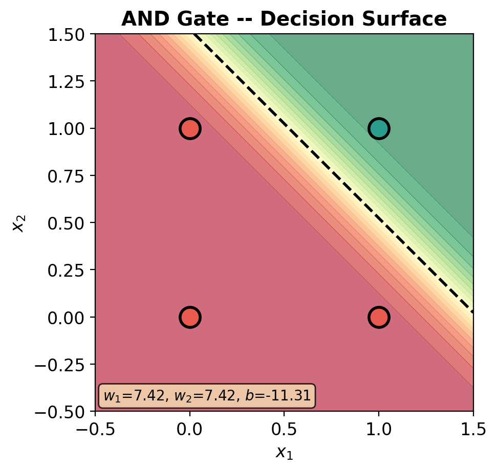
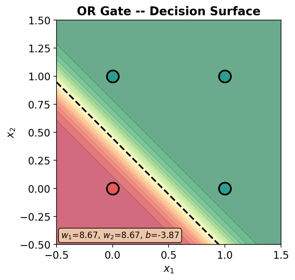
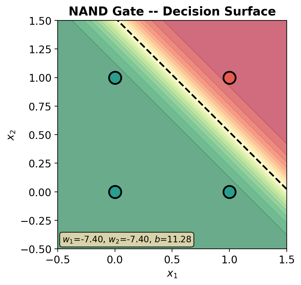
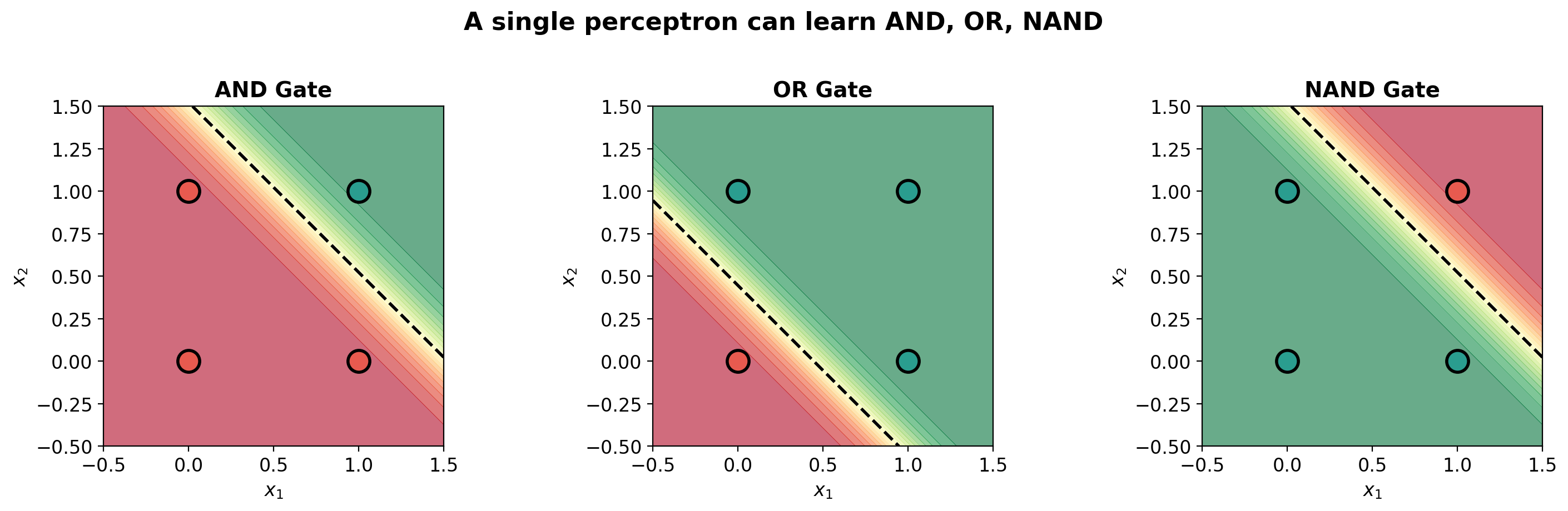
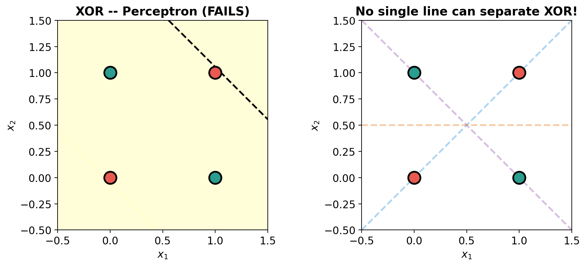
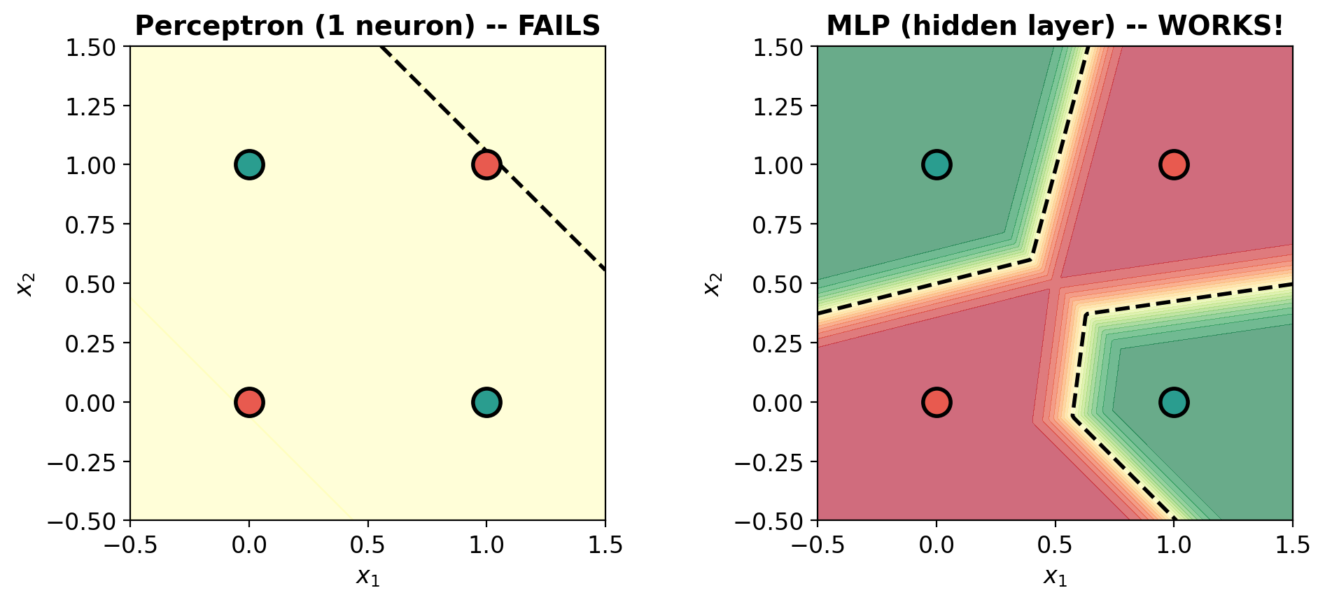
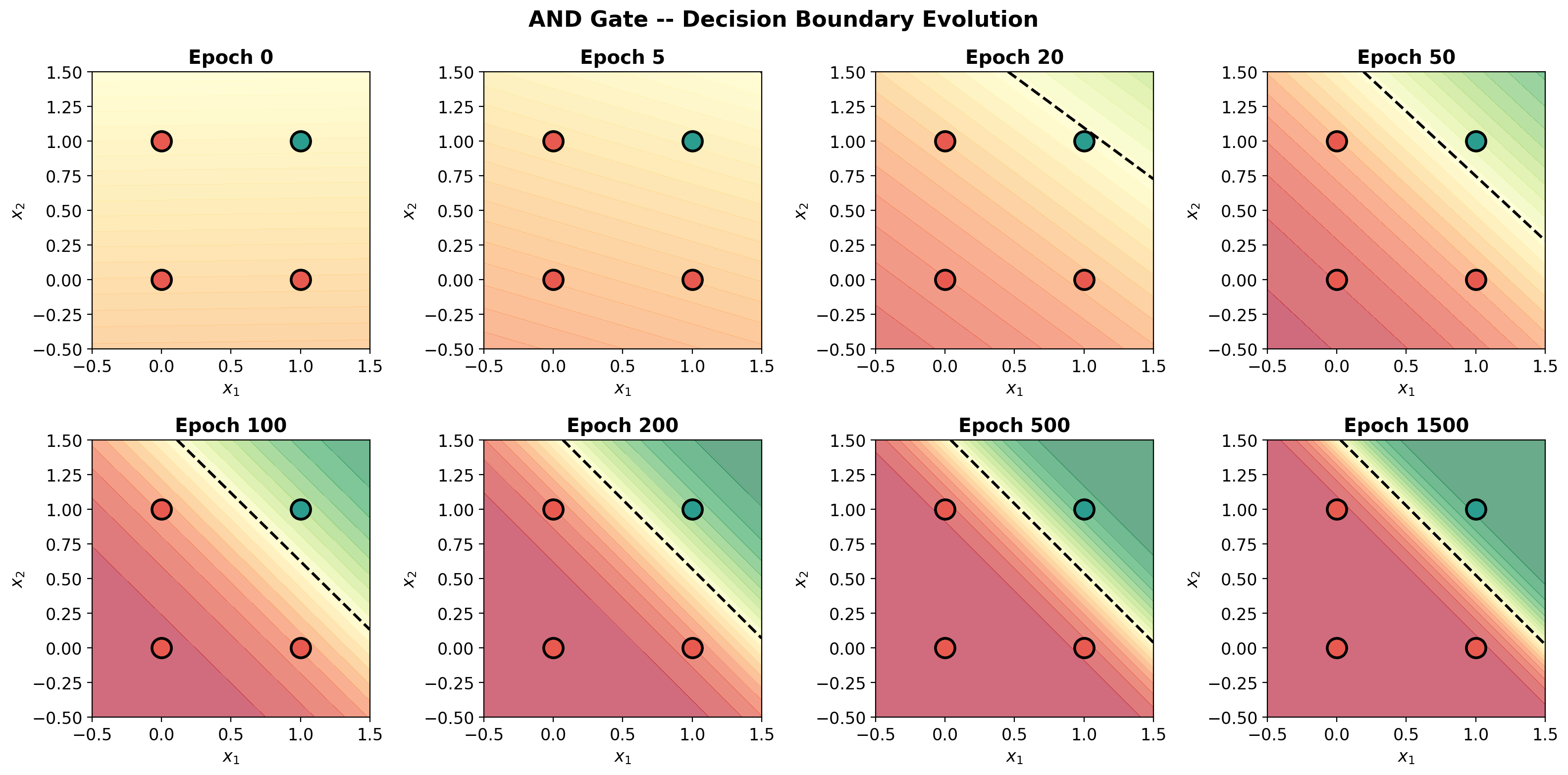
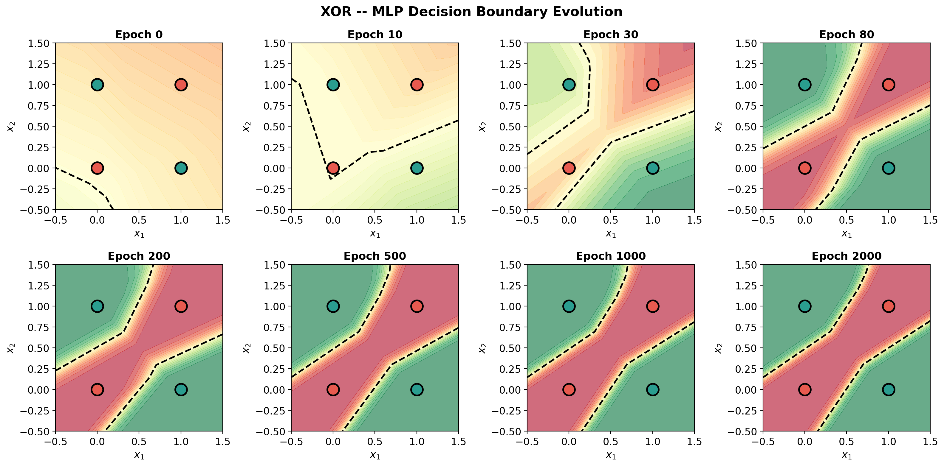
def plot_decision_surface(model, X, y, title='', ax=None):
    """Plot the decision surface of a perceptron."""
    if ax is None:
        fig, ax = plt.subplots(figsize=(5, 5))
    
    # Create mesh
    xx, yy = np.meshgrid(np.linspace(-0.5, 1.5, 200),
                         np.linspace(-0.5, 1.5, 200))
    grid = torch.tensor(np.c_[xx.ravel(), yy.ravel()], dtype=torch.float32)
    
    with torch.no_grad():
        Z = model(grid).numpy().reshape(xx.shape)
    
    # Probability heatmap
    im = ax.contourf(xx, yy, Z, levels=20, cmap='RdYlGn', alpha=0.6, vmin=0, vmax=1)
    ax.contour(xx, yy, Z, levels=[0.5], colors='black', linewidths=2, linestyles='--')
    
    # Data points
    y_np = y.numpy().ravel()
    ax.scatter(X[y_np == 0, 0], X[y_np == 0, 1], c=C0, s=200, edgecolors='black', 
               linewidth=2, zorder=5, label='0')
    ax.scatter(X[y_np == 1, 0], X[y_np == 1, 1], c=C1, s=200, edgecolors='black',
               linewidth=2, zorder=5, label='1')
    
    # Labels on points
    for i in range(len(X)):
        ax.annotate(f'{int(y_np[i])}', (X[i, 0].item(), X[i, 1].item()),
                    ha='center', va='center', fontsize=14, fontweight='bold',
                    color='white' if y_np[i] == 0 else 'white')
    
    ax.set_xlim(-0.5, 1.5); ax.set_ylim(-0.5, 1.5)
    ax.set_xlabel('$x_1$'); ax.set_ylabel('$x_2$')
    ax.set_title(title, fontweight='bold', fontsize=14)
    ax.set_aspect('equal')
    return ax


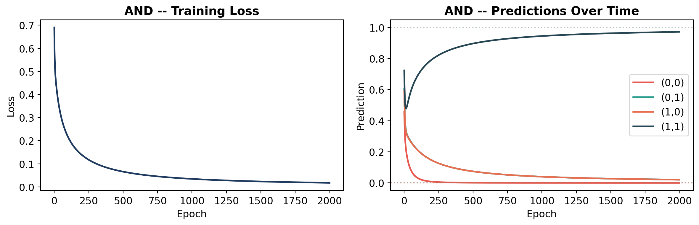
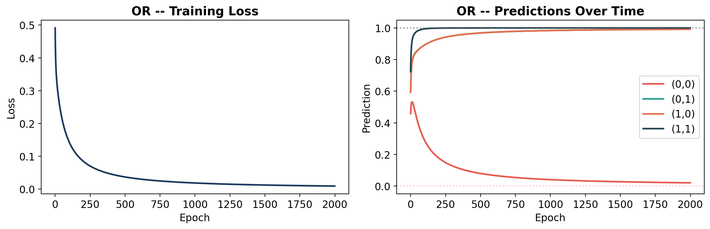
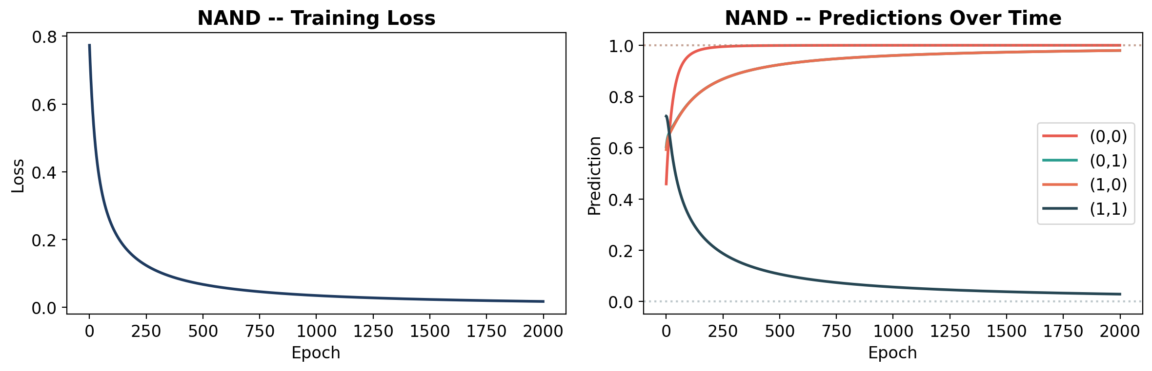
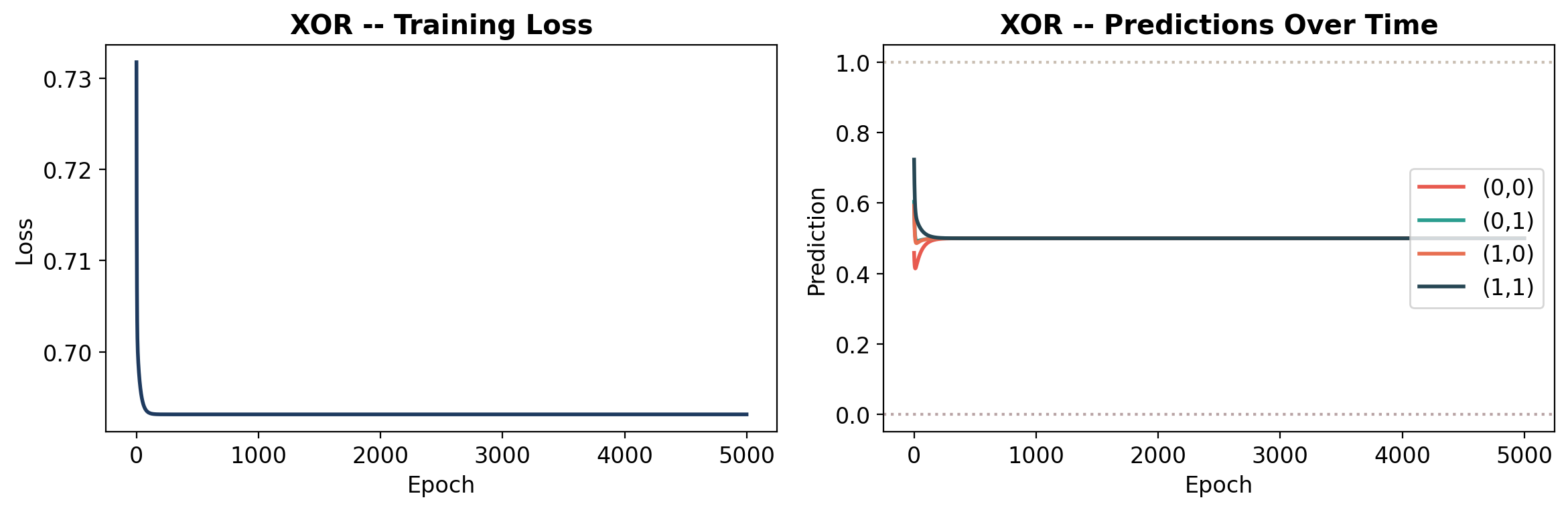
def plot_learning(history, gate_name, y):
    """Plot loss curve and prediction evolution."""
    fig, axes = plt.subplots(1, 2, figsize=(12, 4))
    
    # Loss
    axes[0].plot(history['loss'], color='#1e3a5f', linewidth=2)
    axes[0].set_xlabel('Epoch')
    axes[0].set_ylabel('Loss')
    axes[0].set_title(f'{gate_name} -- Training Loss', fontweight='bold')
    
    # Predictions over time
    preds = np.array(history['predictions'])
    labels = ['(0,0)', '(0,1)', '(1,0)', '(1,1)']
    colors_line = ['#e85a4f', '#2a9d8f', '#e76f51', '#264653']
    for i in range(4):
        axes[1].plot(preds[:, i], label=labels[i], linewidth=2, color=colors_line[i])
    
    # Target lines
    y_np = y.numpy().ravel()
    for i in range(4):
        axes[1].axhline(y=y_np[i], color=colors_line[i], linestyle=':', alpha=0.3)
    
    axes[1].set_xlabel('Epoch')
    axes[1].set_ylabel('Prediction')
    axes[1].set_title(f'{gate_name} -- Predictions Over Time', fontweight='bold')
    axes[1].legend(loc='center right')
    axes[1].set_ylim(-0.05, 1.05)
    
    plt.tight_layout()
    plt.show()

Learning the AND Gate

model_and, hist_and = train_perceptron(X_gate, gates['AND'])

# Show results
plot_learning(hist_and, 'AND', gates['AND'])

# Final predictions
with torch.no_grad():
    preds = model_and(X_gate)
print('Final predictions:')
for i in range(4):
    x1, x2 = int(X_gate[i, 0]), int(X_gate[i, 1])
    p = preds[i].item()
    target = int(gates['AND'][i].item())
    print(f'  {x1} AND {x2} = {p:.3f} (round to {round(p)}) -- target: {target}')

Final predictions:
  0 AND 0 = 0.000 (round to 0) -- target: 0
  0 AND 1 = 0.020 (round to 0) -- target: 0
  1 AND 0 = 0.020 (round to 0) -- target: 0
  1 AND 1 = 0.972 (round to 1) -- target: 1
fig, ax = plt.subplots(figsize=(5, 5))
plot_decision_surface(model_and, X_gate.numpy(), gates['AND'], 'AND Gate -- Decision Surface', ax=ax)

# Show learned weights
w1, w2 = model_and.linear.weight.data.numpy().ravel()
b = model_and.linear.bias.data.item()
ax.text(0.02, 0.02, f'$w_1$={w1:.2f}, $w_2$={w2:.2f}, $b$={b:.2f}',
        transform=ax.transAxes, fontsize=10, verticalalignment='bottom',
        bbox=dict(boxstyle='round', facecolor='wheat', alpha=0.8))
plt.tight_layout()
plt.show()

print(f'Decision boundary: {w1:.2f}*x1 + {w2:.2f}*x2 + {b:.2f} = 0')
print('The line separates (1,1) from everything else.')

Decision boundary: 7.42*x1 + 7.42*x2 + -11.31 = 0
The line separates (1,1) from everything else.

Learning the OR Gate

model_or, hist_or = train_perceptron(X_gate, gates['OR'])
plot_learning(hist_or, 'OR', gates['OR'])

with torch.no_grad():
    preds = model_or(X_gate)
print('Final predictions:')
for i in range(4):
    x1, x2 = int(X_gate[i, 0]), int(X_gate[i, 1])
    p = preds[i].item()
    print(f'  {x1} OR {x2} = {p:.3f} (round to {round(p)}) -- target: {int(gates["OR"][i].item())}')

Final predictions:
  0 OR 0 = 0.020 (round to 0) -- target: 0
  0 OR 1 = 0.992 (round to 1) -- target: 1
  1 OR 0 = 0.992 (round to 1) -- target: 1
  1 OR 1 = 1.000 (round to 1) -- target: 1
fig, ax = plt.subplots(figsize=(5, 5))
plot_decision_surface(model_or, X_gate.numpy(), gates['OR'], 'OR Gate -- Decision Surface', ax=ax)
w1, w2 = model_or.linear.weight.data.numpy().ravel()
b = model_or.linear.bias.data.item()
ax.text(0.02, 0.02, f'$w_1$={w1:.2f}, $w_2$={w2:.2f}, $b$={b:.2f}',
        transform=ax.transAxes, fontsize=10, verticalalignment='bottom',
        bbox=dict(boxstyle='round', facecolor='wheat', alpha=0.8))
plt.tight_layout()
plt.show()

print('The line separates (0,0) from everything else.')

The line separates (0,0) from everything else.

Learning the NAND Gate

model_nand, hist_nand = train_perceptron(X_gate, gates['NAND'])
plot_learning(hist_nand, 'NAND', gates['NAND'])

with torch.no_grad():
    preds = model_nand(X_gate)
print('Final predictions:')
for i in range(4):
    x1, x2 = int(X_gate[i, 0]), int(X_gate[i, 1])
    p = preds[i].item()
    print(f'  {x1} NAND {x2} = {p:.3f} (round to {round(p)}) -- target: {int(gates["NAND"][i].item())}')

Final predictions:
  0 NAND 0 = 1.000 (round to 1) -- target: 1
  0 NAND 1 = 0.980 (round to 1) -- target: 1
  1 NAND 0 = 0.980 (round to 1) -- target: 1
  1 NAND 1 = 0.028 (round to 0) -- target: 0
fig, ax = plt.subplots(figsize=(5, 5))
plot_decision_surface(model_nand, X_gate.numpy(), gates['NAND'], 'NAND Gate -- Decision Surface', ax=ax)
w1, w2 = model_nand.linear.weight.data.numpy().ravel()
b = model_nand.linear.bias.data.item()
ax.text(0.02, 0.02, f'$w_1$={w1:.2f}, $w_2$={w2:.2f}, $b$={b:.2f}',
        transform=ax.transAxes, fontsize=10, verticalalignment='bottom',
        bbox=dict(boxstyle='round', facecolor='wheat', alpha=0.8))
plt.tight_layout()
plt.show()

All Learnable Gates Side by Side

fig, axes = plt.subplots(1, 3, figsize=(15, 4.5))

models = [model_and, model_or, model_nand]
names = ['AND', 'OR', 'NAND']
gate_labels = [gates['AND'], gates['OR'], gates['NAND']]

for ax, model, name, y in zip(axes, models, names, gate_labels):
    plot_decision_surface(model, X_gate.numpy(), y, f'{name} Gate', ax=ax)

plt.suptitle('A single perceptron can learn AND, OR, NAND', fontsize=16, fontweight='bold', y=1.02)
plt.tight_layout()
plt.show()

print('All three gates are linearly separable -- one line does the job.')
print('The perceptron just needs to find the right line.')

All three gates are linearly separable -- one line does the job.
The perceptron just needs to find the right line.

XOR: The Perceptron’s Kryptonite

XOR = 1 when inputs are different, 0 when inputs are the same.

Can a single line separate (0,1) and (1,0) from (0,0) and (1,1)?

model_xor, hist_xor = train_perceptron(X_gate, gates['XOR'], epochs=5000)
plot_learning(hist_xor, 'XOR', gates['XOR'])

with torch.no_grad():
    preds = model_xor(X_gate)

print('Final predictions:')
correct = 0
for i in range(4):
    x1, x2 = int(X_gate[i, 0]), int(X_gate[i, 1])
    p = preds[i].item()
    target = int(gates['XOR'][i].item())
    match = 'OK' if round(p) == target else 'WRONG'
    if round(p) == target: correct += 1
    print(f'  {x1} XOR {x2} = {p:.3f} (round to {round(p)}) -- target: {target}  {match}')

print(f'\nAccuracy: {correct}/4')
print('The perceptron CANNOT learn XOR!')

Final predictions:
  0 XOR 0 = 0.500 (round to 0) -- target: 0  OK
  0 XOR 1 = 0.500 (round to 0) -- target: 1  WRONG
  1 XOR 0 = 0.500 (round to 0) -- target: 1  WRONG
  1 XOR 1 = 0.500 (round to 0) -- target: 0  OK

Accuracy: 2/4
The perceptron CANNOT learn XOR!
fig, axes = plt.subplots(1, 2, figsize=(10, 4.5))

plot_decision_surface(model_xor, X_gate.numpy(), gates['XOR'], 
                      'XOR -- Perceptron (FAILS)', ax=axes[0])

# Show WHY it fails -- the 4 points with no valid line
ax = axes[1]
y_xor = gates['XOR'].numpy().ravel()
ax.scatter(X_gate[y_xor == 0, 0], X_gate[y_xor == 0, 1], c=C0, s=200,
           edgecolors='black', linewidth=2, zorder=5)
ax.scatter(X_gate[y_xor == 1, 0], X_gate[y_xor == 1, 1], c=C1, s=200,
           edgecolors='black', linewidth=2, zorder=5)

for i in range(4):
    ax.annotate(f'{int(y_xor[i])}', (X_gate[i, 0].item(), X_gate[i, 1].item()),
                ha='center', va='center', fontsize=14, fontweight='bold', color='white')

# Try drawing some lines
x_line = np.linspace(-0.5, 1.5, 100)
for slope, intercept, color in [(1, 0, '#3498db'), (-1, 1, '#9b59b6'), (0, 0.5, '#e67e22')]:
    ax.plot(x_line, slope * x_line + intercept, color=color, alpha=0.4, linewidth=2, linestyle='--')

ax.set_xlim(-0.5, 1.5); ax.set_ylim(-0.5, 1.5)
ax.set_xlabel('$x_1$'); ax.set_ylabel('$x_2$')
ax.set_title('No single line can separate XOR!', fontweight='bold', fontsize=14)
ax.set_aspect('equal')

plt.tight_layout()
plt.show()

print('XOR is NOT linearly separable.')
print('No matter what w1, w2, b you pick, one line cannot do it.')

XOR is NOT linearly separable.
No matter what w1, w2, b you pick, one line cannot do it.

The Fix: Add More Neurons (MLP)

One neuron = one line. Two neurons = two lines. Combine them and XOR is solved.

# MLP with one hidden layer (2 hidden neurons)
torch.manual_seed(42)
mlp_xor = nn.Sequential(
    nn.Linear(2, 4),
    nn.ReLU(),
    nn.Linear(4, 1),
    nn.Sigmoid()
)

optimizer = optim.Adam(mlp_xor.parameters(), lr=0.05)
loss_fn = nn.BCELoss()

losses = []
for epoch in range(2000):
    pred = mlp_xor(X_gate)
    loss = loss_fn(pred, gates['XOR'])
    optimizer.zero_grad()
    loss.backward()
    optimizer.step()
    losses.append(loss.item())

with torch.no_grad():
    preds = mlp_xor(X_gate)

print('MLP predictions for XOR:')
for i in range(4):
    x1, x2 = int(X_gate[i, 0]), int(X_gate[i, 1])
    p = preds[i].item()
    target = int(gates['XOR'][i].item())
    print(f'  {x1} XOR {x2} = {p:.3f} (round to {round(p)}) -- target: {target}')

print('\nThe MLP solves XOR!')
MLP predictions for XOR:
  0 XOR 0 = 0.000 (round to 0) -- target: 0
  0 XOR 1 = 1.000 (round to 1) -- target: 1
  1 XOR 0 = 0.999 (round to 1) -- target: 1
  1 XOR 1 = 0.000 (round to 0) -- target: 0

The MLP solves XOR!
# Side by side: Perceptron vs MLP on XOR
fig, axes = plt.subplots(1, 2, figsize=(10, 4.5))

plot_decision_surface(model_xor, X_gate.numpy(), gates['XOR'],
                      'Perceptron (1 neuron) -- FAILS', ax=axes[0])

# MLP decision surface
xx, yy = np.meshgrid(np.linspace(-0.5, 1.5, 200), np.linspace(-0.5, 1.5, 200))
grid = torch.tensor(np.c_[xx.ravel(), yy.ravel()], dtype=torch.float32)
with torch.no_grad():
    Z = mlp_xor(grid).numpy().reshape(xx.shape)

ax = axes[1]
ax.contourf(xx, yy, Z, levels=20, cmap='RdYlGn', alpha=0.6, vmin=0, vmax=1)
ax.contour(xx, yy, Z, levels=[0.5], colors='black', linewidths=2, linestyles='--')
y_xor = gates['XOR'].numpy().ravel()
ax.scatter(X_gate[y_xor == 0, 0], X_gate[y_xor == 0, 1], c=C0, s=200,
           edgecolors='black', linewidth=2, zorder=5)
ax.scatter(X_gate[y_xor == 1, 0], X_gate[y_xor == 1, 1], c=C1, s=200,
           edgecolors='black', linewidth=2, zorder=5)
for i in range(4):
    ax.annotate(f'{int(y_xor[i])}', (X_gate[i, 0].item(), X_gate[i, 1].item()),
                ha='center', va='center', fontsize=14, fontweight='bold', color='white')
ax.set_xlim(-0.5, 1.5); ax.set_ylim(-0.5, 1.5)
ax.set_xlabel('$x_1$'); ax.set_ylabel('$x_2$')
ax.set_title('MLP (hidden layer) -- WORKS!', fontweight='bold', fontsize=14)
ax.set_aspect('equal')

plt.tight_layout()
plt.show()

print('One neuron draws one line. Multiple neurons draw multiple lines.')
print('This is why we need hidden layers!')

One neuron draws one line. Multiple neurons draw multiple lines.
This is why we need hidden layers!

Watching the Decision Boundary Evolve

Let’s watch learning happen in real-time – how the decision boundary moves during training.

First for the AND gate (perceptron), then for XOR (MLP).

# Train AND gate and capture snapshots
torch.manual_seed(0)
model_anim = Perceptron()
optimizer = optim.SGD(model_anim.parameters(), lr=0.5)
loss_fn = nn.BCELoss()

snapshots = []
snapshot_epochs = [0, 5, 20, 50, 100, 200, 500, 1500]

for epoch in range(1501):
    if epoch in snapshot_epochs:
        # Save a snapshot
        snapshots.append({
            'epoch': epoch,
            'w': model_anim.linear.weight.data.clone(),
            'b': model_anim.linear.bias.data.clone(),
            'state': {k: v.clone() for k, v in model_anim.state_dict().items()}
        })
    
    pred = model_anim(X_gate)
    loss = loss_fn(pred, gates['AND'])
    optimizer.zero_grad()
    loss.backward()
    optimizer.step()

# Plot snapshots
fig, axes = plt.subplots(2, 4, figsize=(16, 8))
axes = axes.ravel()

for idx, snap in enumerate(snapshots):
    ax = axes[idx]
    
    # Load snapshot weights
    temp_model = Perceptron()
    temp_model.load_state_dict(snap['state'])
    
    plot_decision_surface(temp_model, X_gate.numpy(), gates['AND'],
                          f'Epoch {snap["epoch"]}', ax=ax)

plt.suptitle('AND Gate -- Decision Boundary Evolution', fontsize=16, fontweight='bold')
plt.tight_layout()
plt.show()

print('The line starts random and gradually moves to separate the classes.')
print('This is gradient descent in action!')

The line starts random and gradually moves to separate the classes.
This is gradient descent in action!

XOR with MLP – Watch the Boundary Become Non-Linear

The MLP learns to draw a curved boundary that separates XOR. Watch it evolve from random to correct.

# Train MLP on XOR and capture snapshots
torch.manual_seed(42)
mlp_anim = nn.Sequential(
    nn.Linear(2, 8),
    nn.ReLU(),
    nn.Linear(8, 1),
    nn.Sigmoid()
)

optimizer = optim.Adam(mlp_anim.parameters(), lr=0.05)
loss_fn = nn.BCELoss()

mlp_snapshots = []
mlp_snapshot_epochs = [0, 10, 30, 80, 200, 500, 1000, 2000]

for epoch in range(2001):
    if epoch in mlp_snapshot_epochs:
        mlp_snapshots.append({
            'epoch': epoch,
            'state': {k: v.clone() for k, v in mlp_anim.state_dict().items()}
        })
    
    pred = mlp_anim(X_gate)
    loss = loss_fn(pred, gates['XOR'])
    optimizer.zero_grad()
    loss.backward()
    optimizer.step()

# Plot snapshots
fig, axes = plt.subplots(2, 4, figsize=(16, 8))
axes_flat = axes.ravel()

xx, yy = np.meshgrid(np.linspace(-0.5, 1.5, 200), np.linspace(-0.5, 1.5, 200))
grid_t = torch.tensor(np.c_[xx.ravel(), yy.ravel()], dtype=torch.float32)
y_xor = gates['XOR'].numpy().ravel()

for idx, snap in enumerate(mlp_snapshots):
    ax = axes_flat[idx]
    
    # Load snapshot
    temp_mlp = nn.Sequential(nn.Linear(2, 8), nn.ReLU(), nn.Linear(8, 1), nn.Sigmoid())
    temp_mlp.load_state_dict(snap['state'])
    
    with torch.no_grad():
        Z = temp_mlp(grid_t).numpy().reshape(xx.shape)
    
    ax.contourf(xx, yy, Z, levels=20, cmap='RdYlGn', alpha=0.6, vmin=0, vmax=1)
    ax.contour(xx, yy, Z, levels=[0.5], colors='black', linewidths=2, linestyles='--')
    
    ax.scatter(X_gate[y_xor == 0, 0], X_gate[y_xor == 0, 1], c=C0, s=200,
               edgecolors='black', linewidth=2, zorder=5)
    ax.scatter(X_gate[y_xor == 1, 0], X_gate[y_xor == 1, 1], c=C1, s=200,
               edgecolors='black', linewidth=2, zorder=5)
    for i in range(4):
        ax.annotate(f'{int(y_xor[i])}', (X_gate[i, 0].item(), X_gate[i, 1].item()),
                    ha='center', va='center', fontsize=14, fontweight='bold', color='white')
    
    ax.set_xlim(-0.5, 1.5); ax.set_ylim(-0.5, 1.5)
    ax.set_xlabel('$x_1$'); ax.set_ylabel('$x_2$')
    ax.set_title(f'Epoch {snap["epoch"]}', fontweight='bold', fontsize=13)
    ax.set_aspect('equal')

plt.suptitle('XOR -- MLP Decision Boundary Evolution', fontsize=16, fontweight='bold')
plt.tight_layout()
plt.show()

print('The boundary starts as a simple line (random weights).')
print('Gradually it bends and curves to separate the diagonal points.')
print('This is the hidden layer learning a non-linear transformation!')

The boundary starts as a simple line (random weights).
Gradually it bends and curves to separate the diagonal points.
This is the hidden layer learning a non-linear transformation!

Summary

Gate Linearly Separable? Perceptron Learns It?
AND Yes Yes
OR Yes Yes
NAND Yes Yes
XOR No No

Key lessons: 1. A perceptron = one neuron = one straight line 2. It learns by adjusting \(w_1, w_2, b\) to minimize loss (gradient descent) 3. If data is linearly separable, the perceptron will find the line 4. XOR is NOT linearly separable – you need multiple neurons (an MLP) 5. This is why neural networks have hidden layers

Minsky & Papert showed this limitation in 1969. It took until the 1980s (backpropagation) to train multi-layer networks effectively.