quizforge / gallery / ec101-demo
Quiz 1 — Markets & Elasticity
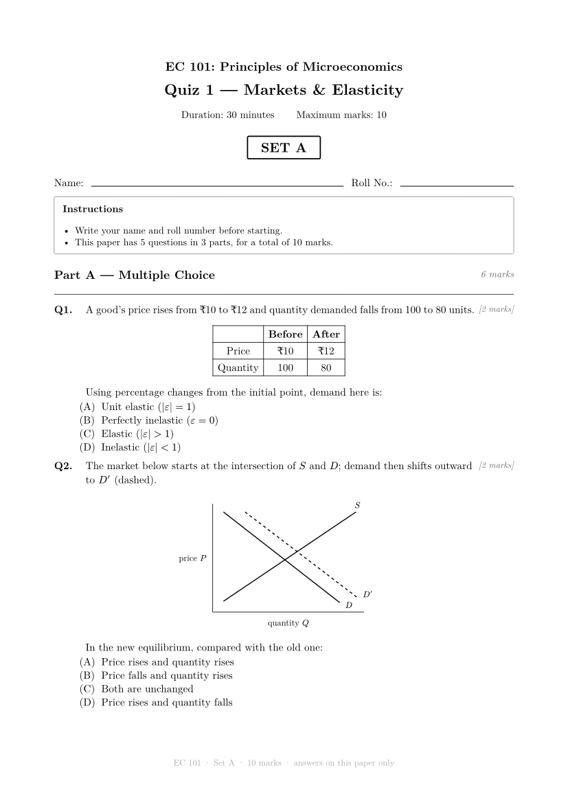
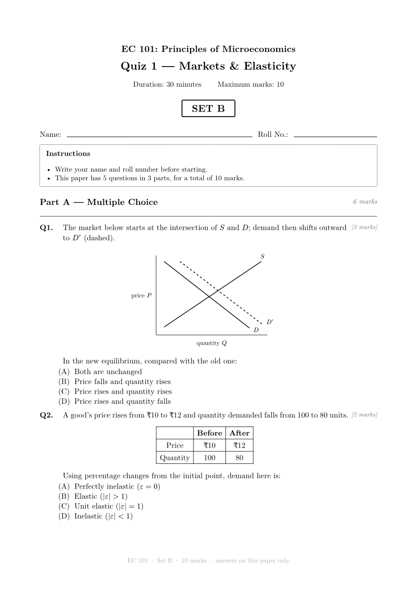
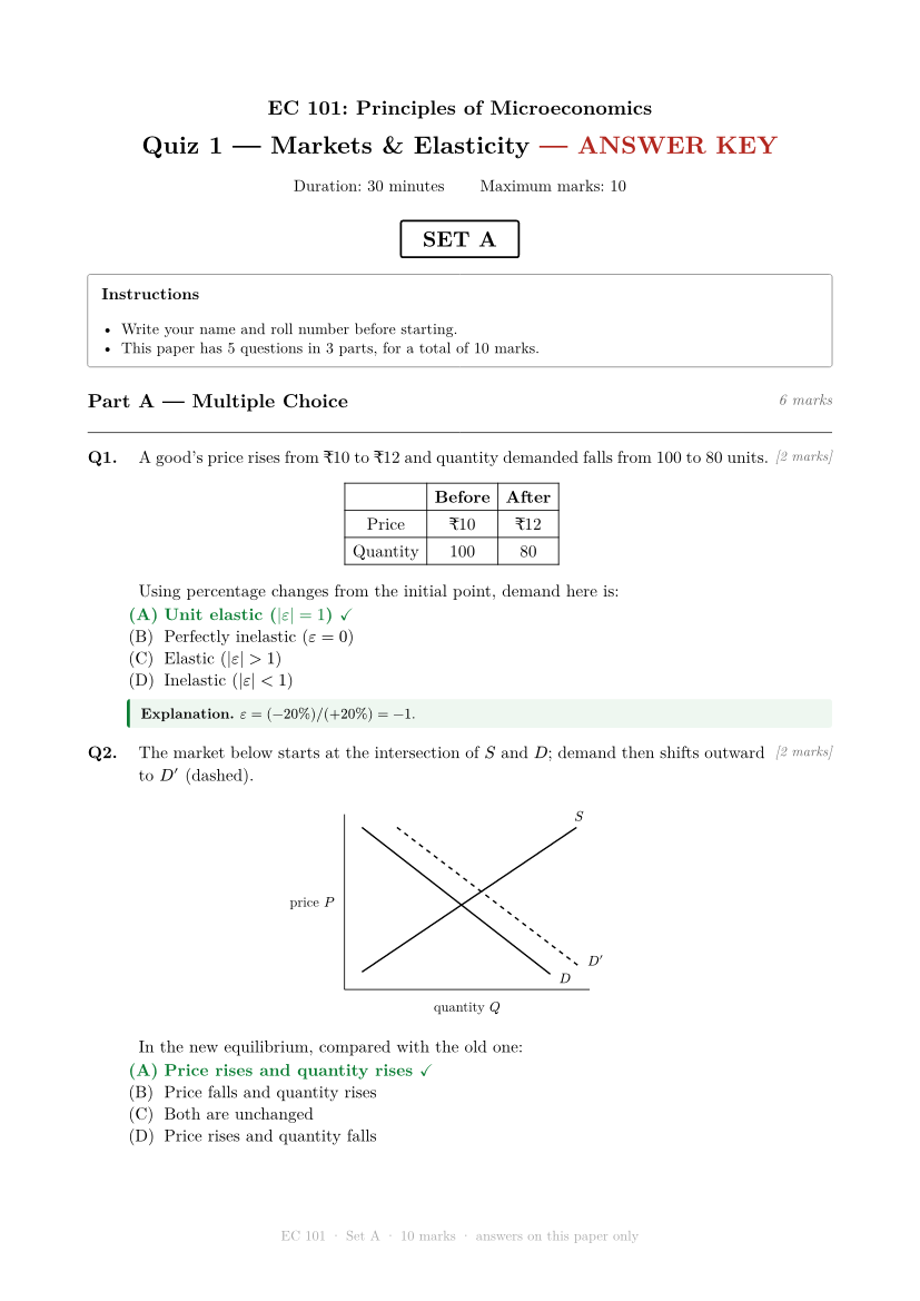
Supply–demand figure, elasticity from a table, an essay — plus a custom footer. Every set below contains exactly the same questions and total marks — only the question order and the MCQ option order differ, derived deterministically from the exam id and the set id.
The 2 versions
Answer key (set A)
The source that generated all of this
One file produces every version above, its keys, and the grading CSV. The feature tour explains each marker with minimal code.
View exams/demo-economics.typ (90 lines)
// Subject demo: microeconomics — a supply/demand figure, an elasticity
// computation from a table, an essay with rubric. Also demonstrates custom
// page furniture (footer:).

#import "/quizforge/lib.typ": *

#let sd-fig = {
  let w = 5.6cm
  let h = 4cm
  align(center, box(width: w + 1.9cm, height: h + 1cm, inset: (left: 1.3cm, bottom: 0.7cm, top: 0.3cm, right: 0.6cm), {
    place(bottom + left, line(length: w, stroke: 0.6pt))
    place(bottom + left, line(angle: -90deg, length: h, stroke: 0.6pt))
    place(bottom + center, dy: 0.5cm, text(size: 9pt, [quantity $Q$]))
    place(left + horizon, dx: -1.25cm, text(size: 9pt, [price $P$]))
    // supply: rising
    place(bottom + left, line(start: (0.4cm, -0.4cm), end: (w - 0.3cm, -h + 0.3cm), stroke: 1pt))
    place(bottom + left, dx: w - 0.35cm, dy: -h + 0.15cm, text(size: 9pt, [$S$]))
    // demand: falling, plus shifted D'
    place(bottom + left, line(start: (0.4cm, -h + 0.3cm), end: (w - 0.9cm, -0.35cm), stroke: 1pt))
    place(bottom + left, dx: w - 0.7cm, dy: -0.15cm, text(size: 9pt, [$D$]))
    place(bottom + left, line(start: (1.2cm, -h + 0.3cm), end: (w - 0.2cm, -0.5cm), stroke: (thickness: 1pt, dash: "dashed")))
    place(bottom + left, dx: w - 0.05cm, dy: -0.55cm, text(size: 9pt, [$D'$]))
  }))
}

#show: quiz.with(
  id: "ec101-demo",
  course: "EC 101: Principles of Microeconomics",
  title: "Quiz 1 — Markets & Elasticity",
  duration: "30 minutes",
  sets: ("A", "B"),
  footer: info => align(
    center,
    text(size: 9pt, fill: gray, [EC 101 · Set #info.at("set") · #info.total marks · answers on this paper only]),
  ),
)

= Multiple Choice

+ #m(2) The market below starts at the intersection of $S$ and $D$; demand
  then shifts outward to $D'$ (dashed).
  #sd-fig
  In the new equilibrium, compared with the old one:
  - ✓ Price rises and quantity rises
  - Price falls and quantity rises
  - Price rises and quantity falls
  - Both are unchanged

+ #m(2) A good's price rises from ₹10 to ₹12 and quantity demanded falls from
  100 to 80 units.
  #align(center, table(
    columns: 3, align: center, stroke: 0.6pt, inset: 5pt,
    [], [*Before*], [*After*],
    [Price], [₹10], [₹12],
    [Quantity], [100], [80],
  ))
  Using percentage changes from the initial point, demand here is:
  - ✓ Unit elastic ($|epsilon| = 1$)
  - Inelastic ($|epsilon| < 1$)
  - Elastic ($|epsilon| > 1$)
  - Perfectly inelastic ($epsilon = 0$)
  #explain[$epsilon = (-20%) \/ (+20%) = -1$.]

+ #m(2) You skip a concert ticket worth ₹500 (which you value at ₹800) to work
  a shift paying ₹600. The opportunity cost of working is:
  - ✓ ₹300 of net enjoyment forgone (₹800 value − ₹500 price)
  - ₹500
  - ₹800
  - ₹600

= Fill in the Blanks

+ #m(1) GDP deflator $=$ (nominal GDP $\/$ real GDP) $times$
  #blank(width: 1.5cm)[100].

= Essay

+ #m(3) "A binding minimum wage always reduces total employment." Discuss in
  at most one page, referencing both the competitive model and one situation
  where the claim can fail.
  #answer(8cm, rubric: [+1 competitive model: wage floor above equilibrium
    → surplus of labor; +1 monopsony (or search friction) counter-case;
    +1 clarity and a stated conclusion.])[
    In the competitive model a binding floor raises wages above equilibrium
    and reduces employment along the demand curve. Under monopsony, however,
    employers face an upward-sloping labor supply and restrict hiring; a
    moderate minimum wage can *increase* employment toward the competitive
    level. Empirical work (e.g. Card–Krueger) suggests small effects near
    current levels.]