quizforge / gallery / es335-2023-archive
Quiz — Trees, Metrics & Ensembles (2023 archive)
Real 2023 course questions ported verbatim: data tables, block quotes, fractional marks. Every set below contains exactly the same questions and total marks — only the question order and the MCQ option order differ, derived deterministically from the exam id and the set id.
The 4 versions
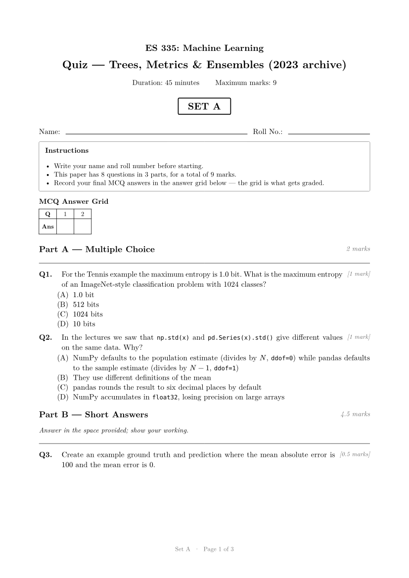
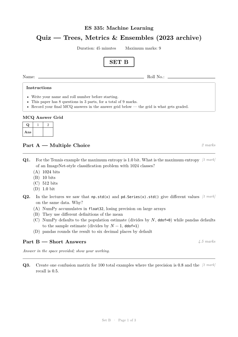
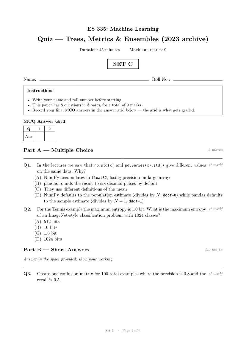

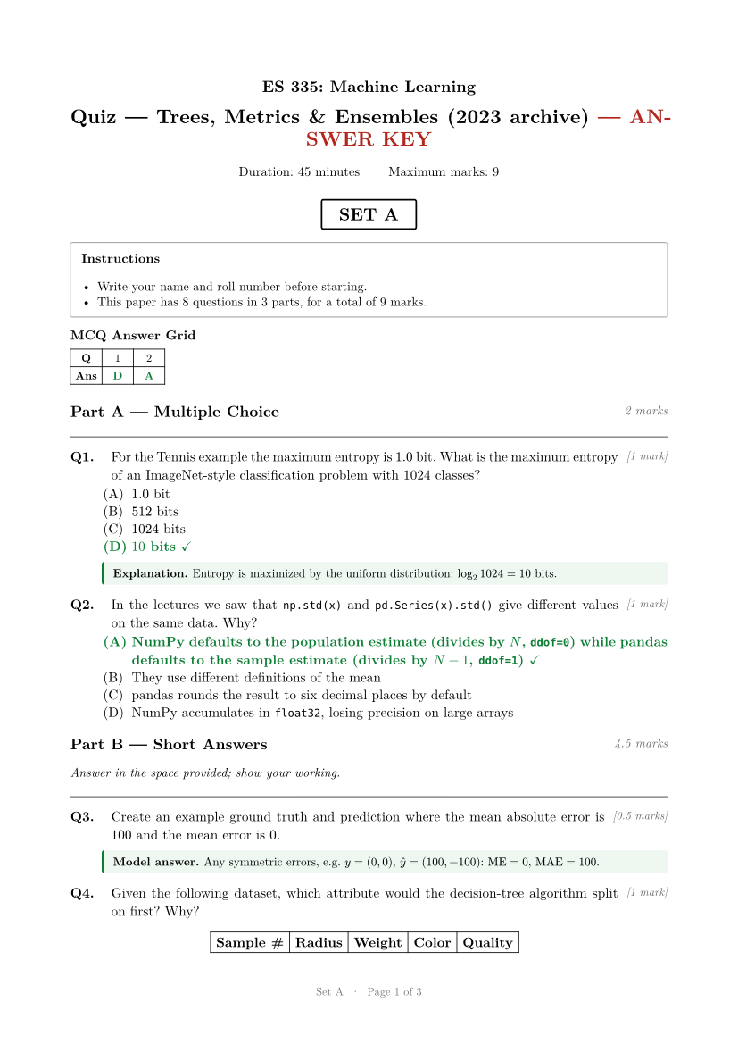
Answer key (set A)
The source that generated all of this
One file produces every version above, its keys, and the grading CSV. The feature tour explains each marker with minimal code.
View exams/quiz4-ml23.typ (120 lines)
// Ported from real ES 335 (Machine Learning) 2023 papers — a subset of
// Quiz 1 (18 Jan: trees, metrics) and Quiz 2 (8 Feb: ensembles), converted
// from Quarto/Markdown to quizforge markup. Model answers added for the key.
//
//   python3 scripts/build.py exams/quiz4-ml23.typ

#import "/quizforge/lib.typ": *

#show: quiz.with(
  id: "es335-2023-archive",
  course: "ES 335: Machine Learning",
  title: "Quiz — Trees, Metrics & Ensembles (2023 archive)",
  duration: "45 minutes",
  sets: ("A", "B", "C", "D"),
  answer-grid: true,
)

= Multiple Choice

+ #m(1) For the Tennis example the maximum entropy is $1.0$ bit. What is the
  maximum entropy of an ImageNet-style classification problem with 1024 classes?
  - ✓ $10$ bits
  - $1.0$ bit
  - $1024$ bits
  - $512$ bits
  #explain[Entropy is maximized by the uniform distribution:
    $log_2 1024 = 10$ bits.]

+ #m(1) In the lectures we saw that `np.std(x)` and `pd.Series(x).std()` give
  different values on the same data. Why?
  - ✓ NumPy defaults to the population estimate (divides by $N$, `ddof=0`)
    while pandas defaults to the sample estimate (divides by $N - 1$, `ddof=1`)
  - pandas rounds the result to six decimal places by default
  - NumPy accumulates in `float32`, losing precision on large arrays
  - They use different definitions of the mean

= Short Answers

Answer in the space provided; show your working.

+ #m(1) Given the following dataset, which attribute would the decision-tree
  algorithm split on first? Why?
  #align(center, table(
    columns: 5,
    align: center,
    stroke: 0.6pt,
    inset: 4.5pt,
    [*Sample \#*], [*Radius*], [*Weight*], [*Color*], [*Quality*],
    [1], [1], [1], [1], [Good],
    [2], [1], [1], [2], [Good],
    [3], [1], [2], [1], [Bad],
    [4], [1], [2], [2], [Bad],
    [5], [2], [1], [1], [Good],
    [6], [2], [2], [2], [Good],
  ))
  #answer(5cm, rubric: [+0.5 correct attribute; +0.5 information-gain argument.])[
    Weight. $H("Quality") = H(2\/6) approx 0.918$. Splitting on Weight:
    weight 1 → all Good ($H = 0$); weight 2 → (1 Good, 2 Bad),
    $H approx 0.918$; weighted $approx 0.459$, so $"IG" approx 0.459$ — higher
    than Radius ($"IG" approx 0.25$) and Color ($"IG" = 0$).]

+ #m(2) #qid("xor-prepruning") Quoting Wikipedia:
  #quote(block: true)[Pre-pruning procedures prevent a complete induction of
    the training set by replacing a stop criterion in the induction algorithm
    (e.g.\ maximum tree depth or information gain > minGain).]
  Create a decision tree for the classification problem below, and explain why
  pre-pruning using information gain can be limiting.
  #align(center, table(
    columns: 3,
    align: center,
    stroke: 0.6pt,
    inset: 4.5pt,
    [$x_1$], [$x_2$], [$y$],
    [0], [0], [0],
    [0], [1], [1],
    [1], [0], [1],
    [1], [1], [0],
  ))
  #answer(7cm, rubric: [+1 a correct depth-2 tree (split on $x_1$, then $x_2$);
    +1 argument: both root splits have zero gain, so gain-based pre-pruning
    stops before the informative second level.])[
    This is XOR: splitting on either $x_1$ or $x_2$ alone leaves both children
    at 50/50, so $"IG" = 0$ at the root — gain-based pre-pruning halts
    immediately. Yet the depth-2 tree (split $x_1$, then $x_2$ in each branch)
    classifies perfectly: gain can be zero at one level and large at the next.]

+ #m(0.5) Create an example ground truth and prediction where the mean
  absolute error is $100$ and the mean error is $0$.
  #answer(3cm)[Any symmetric errors, e.g. $y = (0, 0)$,
    $hat(y) = (100, -100)$: $"ME" = 0$, $"MAE" = 100$.]

+ #m(1) Create one confusion matrix for 100 total examples where the precision
  is $0.8$ and the recall is $0.5$.
  #answer(4.5cm, rubric: [+0.5 consistent TP/FP from precision;
    +0.5 FN from recall and a total of 100.])[
    Take $"TP" = 40$: precision $0.8 arrow.r.double "FP" = 10$; recall $0.5
    arrow.r.double "FN" = 40$; then $"TN" = 10$. Total $= 100$.]

= Ensembles #section(shuffle: false)

+ #m(1.5) In bootstrap sampling we sample $N$ times with replacement from an
  original dataset of $N$ distinct elements (e.g. for $N = 8$, a bootstrap
  sample may be ${8, 8, 3, 4, 5, 1, 8, 5}$, which has 5 unique elements).
  Show that on average a bootstrap sample contains $approx 63.2%$ of $N$
  unique elements.
  #answer(6cm, rubric: [+0.5 miss probability $(1 - 1\/N)^N$; +0.5 expected
    unique count $N(1 - (1 - 1\/N)^N)$; +0.5 limit $1 - 1\/e approx 0.632$.])[
    An element is missed by one draw w.p. $1 - 1\/N$, by all $N$ draws w.p.
    $(1 - 1\/N)^N$. Expected unique fraction $= 1 - (1 - 1\/N)^N arrow.r
    1 - 1\/e approx 0.632$ as $N$ grows.]

+ #m(1) Assume $K$ ensemble members, each with the same error probability
  $p < 0.5$. The binomial argument says the ensemble error shrinks as $K$
  grows — yet empirically, adding members may not always reduce the error.
  Why?
  #answer(4cm)[The binomial argument assumes *independent* errors. Members
    trained on similar data make correlated mistakes, so the effective
    ensemble size saturates and errors shared by many members never get
    voted away.]