Quiz 1 — Foundations, Trees & Nearest Neighbours

// Real-course demo: an ES 335-style Machine Learning quiz with figures and
// tables, written entirely in plain markup. Compiled as-is → answer key.
//
//   python3 scripts/build.py exams/quiz3.typ        # all sets + keys + CSV

#import "/quizforge/lib.typ": *

// ---- figures (plain Typst, no packages — grayscale for print) -------------

// kNN scatter: ● class A, □ class B, ⨯ the query point.
#let knn-fig = {
  let w = 5.2cm
  let h = 4.2cm
  let dot(x, y) = place(dx: x * w - 2.2pt, dy: (1 - y) * h - 2.2pt, circle(radius: 2.2pt, fill: black))
  let sq(x, y) = place(dx: x * w - 2.6pt, dy: (1 - y) * h - 2.6pt, rect(width: 5.2pt, height: 5.2pt, stroke: 0.9pt))
  let query(x, y) = place(
    dx: x * w - 4pt, dy: (1 - y) * h - 7.5pt,
    text(size: 13pt, weight: "bold", sym.times),
  )
  align(center, box(width: w + 1.4cm, height: h + 1.1cm, inset: (left: 0.9cm, bottom: 0.7cm, top: 0.4cm, right: 0.5cm), {
    place(bottom + left, line(length: w, stroke: 0.6pt))
    place(bottom + left, line(angle: -90deg, length: h, stroke: 0.6pt))
    place(bottom + center, dy: 0.55cm, text(size: 9pt, [$x_1$]))
    place(left + horizon, dx: -0.75cm, text(size: 9pt, [$x_2$]))
    box(width: w, height: h, {
      // class A cluster (top-left) with two members near the query
      dot(0.18, 0.72); dot(0.30, 0.84); dot(0.52, 0.86); dot(0.32, 0.62); dot(0.36, 0.44)
      // class B cluster (bottom-right) with one stray member nearest the query
      sq(0.62, 0.30); sq(0.70, 0.42); sq(0.80, 0.24); sq(0.66, 0.14); sq(0.86, 0.44)
      sq(0.50, 0.63)
      query(0.44, 0.55)
    })
  }))
}

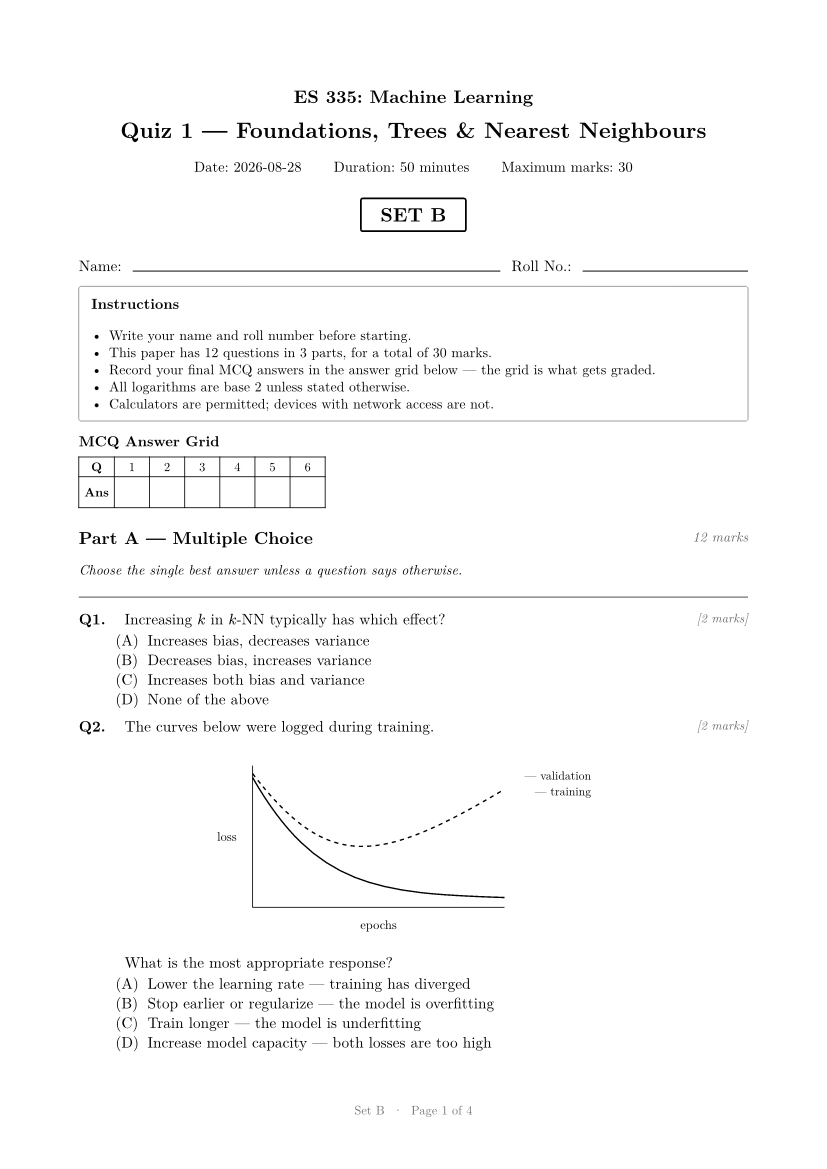
// Loss curves: training loss falls; validation loss falls then rises.
#let loss-fig = {
  let w = 6.4cm
  let h = 3.6cm
  align(center, box(width: w + 3.4cm, height: h + 1.2cm, inset: (left: 1cm, bottom: 0.8cm, top: 0.4cm, right: 2.4cm), {
    place(bottom + left, line(length: w, stroke: 0.6pt))
    place(bottom + left, line(angle: -90deg, length: h, stroke: 0.6pt))
    place(bottom + center, dy: 0.55cm, text(size: 9pt, [epochs]))
    place(left + horizon, dx: -0.9cm, text(size: 9pt, [loss]))
    // training loss (solid): monotone decrease
    place(bottom + left, curve(
      stroke: 1pt,
      curve.move((0cm, -h + 0.3cm)),
      curve.cubic((w * 0.25, -0.5cm), (w * 0.5, -0.35cm), (w, -0.25cm)),
    ))
    // validation loss (dashed): dips at ~40% then rises
    place(bottom + left, curve(
      stroke: (thickness: 1pt, dash: "dashed"),
      curve.move((0cm, -h + 0.2cm)),
      curve.cubic((w * 0.3, -0.9cm), (w * 0.5, -1.1cm), (w, -h + 0.6cm)),
    ))
    place(top + right, dx: 2.2cm, dy: 0.15cm, text(size: 8.5pt, [--- validation \ — training]))
  }))
}

// ---- the paper -------------------------------------------------------------

#show: quiz.with(
  id: "es335-quiz-1",
  course: "ES 335: Machine Learning",
  title: "Quiz 1 — Foundations, Trees & Nearest Neighbours",
  date: "2026-08-28",
  duration: "50 minutes",
  sets: ("A", "B", "C", "D"),
  answer-grid: true,
  instructions: (
    [All logarithms are base 2 unless stated otherwise.],
    [Calculators are permitted; devices with network access are not.],
  ),
)

= Multiple Choice

Choose the single best answer unless a question says otherwise.

+ #m(2) A binary classifier produces the confusion matrix below.
  #align(center, table(
    columns: 3,
    align: center,
    stroke: 0.6pt,
    inset: 5pt,
    [], [*Predicted +*], [*Predicted −*],
    [*Actual +*], [40], [10],
    [*Actual −*], [20], [30],
  ))
  What is its precision?
  - ✓ $40 \/ 60$
  - $40 \/ 50$
  - $40 \/ 100$
  - $70 \/ 100$
  #explain[Precision $= "TP" \/ ("TP" + "FP") = 40 \/ (40 + 20)$. $40\/50$ is the
    recall and $70\/100$ the accuracy.]

+ #m(2) The figure shows training points from two classes and a query point $times$.
  #knn-fig
  Using Euclidean distance, how does the query point get classified by 1-NN and
  by 3-NN respectively?
  - ✓ 1-NN: class B (#sym.square), #h(2pt) 3-NN: class A (#sym.circle.filled)
  - 1-NN: class A (#sym.circle.filled), #h(2pt) 3-NN: class A (#sym.circle.filled)
  - 1-NN: class B (#sym.square), #h(2pt) 3-NN: class B (#sym.square)
  - 1-NN: class A (#sym.circle.filled), #h(2pt) 3-NN: tie
  #explain[The single nearest neighbour is the stray #sym.square just above the
    query; the 3-neighbourhood contains two #sym.circle.filled and one #sym.square.]

+ #m(2) Increasing $k$ in $k$-NN typically has which effect?
  - ✓ Increases bias, decreases variance
  - Decreases bias, increases variance
  - Increases both bias and variance
  - None of the above
  #explain[Larger neighbourhoods average over more points: smoother (higher-bias),
    more stable (lower-variance) decision boundaries.]

+ #m(2) Which of the following objectives are convex in their parameters?
  - ✓ Linear regression with squared loss
  - ✓ Logistic regression negative log-likelihood
  - The $k$-means clustering objective (jointly in assignments and centroids)
  - A two-layer neural network with squared loss
  #explain[Both linear-regression MSE and logistic NLL are convex; $k$-means and
    neural-network losses are not.]

+ #m(2) #qid("es335-loss-curves") The curves below were logged during training.
  #loss-fig
  What is the most appropriate response?
  - ✓ Stop earlier or regularize — the model is overfitting
  - Train longer — the model is underfitting
  - Increase model capacity — both losses are too high
  - Lower the learning rate — training has diverged
  #explain[Training loss keeps falling while validation loss rises after its
    minimum: the classic overfitting signature.]

+ #m(2) #opts(columns: 2) For a split that sends all positives left and all
  negatives right, the weighted entropy of the children is:
  - ✓ $0$
  - $0.5$
  - $1$
  - $log_2 3$

= Fill in the Blanks

+ #m(1) Computing inner products in a high-dimensional feature space without
  ever constructing the features is known as the kernel #blank[trick].

+ #m(1) Compared with L2, L1 regularization tends to produce weight vectors
  that are #blank(width: 3cm)[sparse (many exact zeros)].

+ #m(2) For linear regression in matrix form, the least-squares solution is
  $hat(theta) = (X^top X)^(#blank(width: 1.5cm)[$-1$]) X^top #blank(width: 1.5cm)[$y$]$.

= Long Answers #section(shuffle: false)

Answer in the space provided; show your working.

+ #m(5) The table records eight days of data for predicting whether a match is
  #emph[Played].
  #align(center, table(
    columns: 4,
    align: center,
    stroke: 0.6pt,
    inset: 4.5pt,
    [*Day*], [*Outlook*], [*Windy*], [*Played*],
    [1], [Sunny], [No], [Yes],
    [2], [Sunny], [Yes], [No],
    [3], [Overcast], [No], [Yes],
    [4], [Overcast], [Yes], [Yes],
    [5], [Rainy], [No], [Yes],
    [6], [Rainy], [Yes], [No],
    [7], [Sunny], [No], [No],
    [8], [Rainy], [No], [Yes],
  ))
  Compute (i) the entropy of #emph[Played], and (ii) the information gain of
  splitting on #emph[Windy]. Which single-feature split would a decision tree
  prefer if the gain for #emph[Outlook] is $0.311$?
  #answer(9cm, rubric: [+1 $H("Played")$; +2 conditional entropies; +1 gain;
    +1 correct comparison and conclusion.])[
    $H("Played") = H(5\/8) = -5/8 log 5/8 - 3/8 log 3/8 approx 0.954$.
    Windy = Yes: (1 Yes, 2 No), $H approx 0.918$; Windy = No: (4 Yes, 1 No),
    $H approx 0.722$. Weighted: $3/8 dot 0.918 + 5/8 dot 0.722 approx 0.795$.
    $"IG"("Windy") approx 0.954 - 0.795 = 0.159 < 0.311$, so the tree splits on
    #emph[Outlook].]

+ #m(5) Starting from $L(theta) = norm(y - X theta)_2^2$, derive the normal
  equation. State the condition under which the solution is unique, and give
  one practical remedy when it is not.
  #answer(8cm, rubric: [+2 gradient $-2 X^top (y - X theta)$; +1 setting to zero
    → $X^top X theta = X^top y$; +1 uniqueness ⇔ $X^top X$ invertible (full
    column rank); +1 remedy: ridge / drop collinear features.])[
    $nabla_theta L = -2 X^top (y - X theta) = 0 arrow.r.double X^top X theta =
    X^top y$. Unique iff $X$ has full column rank. Remedy: add ridge penalty
    $lambda I$ (or remove collinear features).]

+ #m(4) Your colleague reports 99.2% accuracy on a fraud-detection dataset in
  which 0.8% of transactions are fraudulent. Explain why this number is not
  impressive, and name two evaluation metrics (or tools) better suited to this
  setting, justifying each in one line.
  #answer(6cm, rubric: [+2 base-rate argument (predicting "not fraud" gives
    99.2%); +1 per metric with justification (max 2): precision/recall, F1,
    PR-AUC, recall at fixed FPR, cost-sensitive evaluation.])[
    A constant "not fraud" classifier already achieves 99.2% — accuracy is
    dominated by the majority class. Better: recall (catch rate of actual
    fraud) with precision or F1 / PR-AUC, which focus on the rare positive
    class rather than overall agreement.]