Previously on CS 203...

The Problem: We need 100,000 labeled movies!

Can we do better?

The Labeling Bottleneck

Traditional Approach: Label everything, then train

Unlabeled Data (100K) → Label ALL → Labeled Data → Train Model

The bottleneck is labeling, not training!

What if we could label smarter instead of labeling everything?

Four Strategies to Reduce Labeling Cost

Today: All four techniques + how to combine them!

What is Active Learning?

Core Idea: Let the model choose which examples to label.

Why it works: Not all examples are equally informative!

The Teaching Analogy

Imagine you're learning to drive:

Active learning focuses effort where it helps most!

Active Learning: The Intuition

Easy Examples (Model is confident → Don't label)

• "I loved this movie! Best film ever!" → Model: 99% POSITIVE
• "Terrible waste of time." → Model: 98% NEGATIVE

Hard Examples (Model is uncertain → LABEL THESE!)

• "The movie was... interesting." → Model: 48% POS, 52% NEG
• "It was okay, I guess." → Model: 51% POS, 49% NEG

Hard examples teach the model the most!

Movie Review Example: Why Uncertainty Matters

# Our movie review classifier after training on 100 examples

reviews = [
    "Best movie ever! 10/10!",           # Model: 99% POS - Already knows this
    "Terrible waste of time.",            # Model: 98% NEG - Already knows this
    "It was okay, I guess.",              # Model: 52% POS - UNCERTAIN!
    "Interesting but flawed.",            # Model: 55% NEG - UNCERTAIN!
    "Not bad, not great.",                # Model: 49% POS - VERY UNCERTAIN!
]

# Which should we label next?
# The uncertain ones! They define the decision boundary.

The model already "knows" extreme reviews. Label the ambiguous ones!

The Decision Boundary Intuition

Example: Classifying handwritten digits 3 vs 5

• Far from boundary → Easy to classify (don't need labels)
• Near boundary → Ambiguous (model confused) → Label these!

Active learning focuses on the decision boundary!

The Active Learning Loop

Repeat until budget exhausted or accuracy target reached

Query Strategies: How to Pick Examples

Model predicts class probabilities → Use them to find informative examples

Three ways to measure "uncertainty":

Visualizing Uncertainty: Binary Case

Both peak at P(+) = 0.5 — maximum uncertainty when model is 50-50!

Query Strategies: 3-Class Comparison

Active Learning: The Algorithm

INPUTS:
  - Small labeled set: L = {(x₁,y₁), ..., (x₁₀,y₁₀)}
  - Large unlabeled pool: U = {x₁, x₂, ..., x₁₀₀₀₀}
  - Query budget: B = 100

ALGORITHM:
  1. Train model M on L
  2. For i = 1 to B:
       a. For each x in U: compute uncertainty(x)
       b. Select x* = argmax uncertainty(x)
       c. Get human label y* for x*
       d. L = L ∪ {(x*, y*)}
       e. U = U \ {x*}
       f. Retrain M on L
  3. Return M

Active Learning: Python Pseudocode

# Initialize
model = RandomForestClassifier()
model.fit(X_labeled, y_labeled)
pool = X_unlabeled.copy()

# Active learning loop
for i in range(budget):
    # 1. Get model's uncertainty on pool
    probs = model.predict_proba(pool)
    uncertainty = 1 - probs.max(axis=1)

    # 2. Select most uncertain example
    query_idx = uncertainty.argmax()

    # 3. Get human label (simulated or real)
    y_new = get_human_label(pool[query_idx])

    # 4. Add to training set & retrain
    X_labeled = np.vstack([X_labeled, pool[query_idx]])
    y_labeled = np.append(y_labeled, y_new)
    pool = np.delete(pool, query_idx, axis=0)
    model.fit(X_labeled, y_labeled)

Active Learning: Typical Results

Batch Active Learning: The Problem

Problem: Querying one at a time is slow. Let's query a batch!

All 5 are uncertain "3 vs 5" — labeling all gives ~same info as labeling 1!

Batch Active Learning: The Solution

Solution: Select diverse uncertain examples

Each example covers a different confusion — each label teaches something new!

Diversity in Batch Selection

Further Reading: BALD (Houlsby et al., 2011), BatchBALD (Kirsch et al., 2019)

Practical Issue 1: Cold Start Problem

Problem: Initial model is bad → uncertainty estimates are meaningless!

Solutions:

• Start with random/stratified sample (10-50 examples)
• Use diversity sampling for first few rounds
• Switch to uncertainty after model stabilizes

Practical Issue 2: When to Stop?

Problem: How do you know when you have enough labels?

Practical tip: Plot learning curve live!

• If accuracy plateaus → stop (more labels won't help)
• If still rising steeply → continue

Practical Issue 3: Class Imbalance

Problem: Uncertainty sampling may ignore rare classes!

What happens: Model never learns rare class well

Solutions:

• Stratified sampling (ensure all classes represented)
• Class-balanced uncertainty (normalize by class frequency)
• Hybrid: uncertainty + random sampling from rare classes

Practical Issue 4: Batch vs Sequential

Practical choice: Almost always use batch!

• Batch size 10-50 is typical
• Retrain every batch (not every label)
• Use diversity to avoid redundant batches

Query By Committee (QBC)

Idea: Train multiple models, query where they disagree

Vote Entropy: 2 POS, 2 NEG → High disagreement → Label this!

When to use: When you can train multiple diverse models cheaply

Active Learning for Regression

Problem: No class probabilities! How to measure uncertainty?

Example: Predicting house prices

→ Query House B — models are uncertain about its price!

Active Learning for Other Tasks

Key Insight: Adapt uncertainty measure to your output structure!

AL for NER: Token-Level Uncertainty

Aggregate strategies: Query sentence if any token is uncertain, or by average uncertainty.

AL for Object Detection

Query images where: detector unsure if object exists, confused about class, or uncertain about box location.

AL for Semantic Segmentation

Query pixels/regions at boundaries — clear sky and buildings don't need more labels!

Bayesian Active Learning

Idea: Use model uncertainty from Bayesian inference

BALD (Bayesian Active Learning by Disagreement):

• Select examples that would most reduce model uncertainty
• Considers both what the model is uncertain about and why

Libraries: baal (Bayesian Active Learning), uncertainty-toolbox

Active Learning Tools

# Install modAL
pip install modAL-python

# Install Label Studio with ML backend
pip install label-studio
pip install label-studio-ml

Weak Supervision: The Big Picture

Write labeling functions (heuristics) → Snorkel combines noisy votes → probabilistic labels

What is Weak Supervision?

Core Idea: Write labeling functions (code) instead of labeling examples.

# Traditional: Label 10,000 examples by hand

# Weak Supervision: Write 10 labeling functions
def lf_contains_love(text):
    return "POSITIVE" if "love" in text.lower() else None

def lf_contains_terrible(text):
    return "NEGATIVE" if "terrible" in text.lower() else None

def lf_exclamation_count(text):
    if text.count("!") > 3:
        return "POSITIVE"
    return None

Trade-off: Labels are noisier, but you get many more of them!

The Expert Knowledge Intuition

You're a movie critic. How do you know a review is positive?

Weak supervision = encoding your expert intuition as code!

Labeling Functions: Netflix Example (using Snorkel)

# Snorkel labeling functions for movie sentiment

@labeling_function()
def lf_high_rating(movie):
    """Movies rated > 8 on IMDB are usually good."""
    if movie.imdb_rating and movie.imdb_rating > 8.0:
        return POSITIVE
    return ABSTAIN

@labeling_function()
def lf_oscar_winner(movie):
    """Oscar winners are good movies."""
    if "Oscar" in str(movie.awards) and "Won" in str(movie.awards):
        return POSITIVE
    return ABSTAIN

@labeling_function()
def lf_low_box_office(movie):
    """Very low box office often means bad movie."""
    if movie.box_office and movie.box_office < 1_000_000:
        return NEGATIVE
    return ABSTAIN

@labeling_function()
def lf_sequel_fatigue(movie):
    """Sequels numbered > 3 are often worse."""
    if re.search(r'\b[4-9]\b|10|11|12', movie.title):
        return NEGATIVE
    return ABSTAIN

Labeling Functions: Characteristics

Key tradeoff: Each LF may be weak alone, but combining many gives coverage + accuracy!

Labeling Functions: Types

1. Keyword/Pattern-based

def lf_keyword_positive(text):
    keywords = ["amazing", "excellent", "loved", "great"]
    return "POS" if any(k in text.lower() for k in keywords) else None

2. Heuristic-based

def lf_short_reviews_negative(text):
    # Short reviews tend to be complaints
    return "NEG" if len(text.split()) < 10 else None

3. External Knowledge

def lf_known_good_movie(text, movie_title):
    top_movies = load_imdb_top_250()
    return "POS" if movie_title in top_movies else None

Labeling Function Conflicts

Problem: LFs often disagree!

text = "I love how terrible this movie is!"

lf_contains_love(text)     # Returns: "POSITIVE"
lf_contains_terrible(text) # Returns: "NEGATIVE"

# Which one is right?

Solution: Use a Label Model to combine LF outputs.

Snorkel: The Weak Supervision Framework

from snorkel.labeling import labeling_function

ABSTAIN, NEGATIVE, POSITIVE = -1, 0, 1

@labeling_function()
def lf_contains_good(x):
    return POSITIVE if "good" in x.text.lower() else ABSTAIN

@labeling_function()
def lf_contains_bad(x):
    return NEGATIVE if "bad" in x.text.lower() else ABSTAIN

@labeling_function()
def lf_high_rating(x):
    return POSITIVE if x.rating > 8 else ABSTAIN

Demo: lecture-demos/week04/snorkel_weak_supervision.py

Worked Example: Our 5 Movie Reviews

Task: Label these 5 reviews as POS/NEG (we don't know true labels!)

2 Labeling Functions:

• LF₁: "good" in text → vote POS (else abstain)
• LF₂: rating > 7 → vote POS; rating < 4 → vote NEG (else abstain)

Step 1: Apply LFs → Label Matrix

Coverage: LF₁ fires on 3/5 = 60%, LF₂ fires on 3/5 = 60%

Step 2: Find Overlaps & Conflicts

Overlap = both LFs vote on same review

#	LF₁	LF₂	Both vote?	Agree?
1	POS	POS	Yes	Yes
2	POS	—	No	—
3	—	NEG	No	—
4	—	POS	No	—
5	POS	—	No	—

Only 1 overlap — not enough to estimate accuracy! Let's scale up...

Step 3a: What is α (Accuracy)?

α = probability that a labeling function is correct when it votes

Problem: We don't know the true labels, so we can't directly compute α!

Snorkel's trick: Estimate α from agreement patterns between LFs.

Step 3b: Scaling to 1000 Reviews

Same LFs applied to 1000 reviews:

Observed agreement rate = 85/100 = 85%

Step 3c: The Agreement Equation

Key insight: When do LF₁ and LF₂ agree on a review?

1. Both correct: LF₁ right AND LF₂ right → probability = α₁ × α₂
2. Both wrong: LF₁ wrong AND LF₂ wrong → probability = (1-α₁) × (1-α₂)

We observed 85% agreement, so:

One equation, two unknowns (α₁, α₂). Need a 3rd LF!

Step 3d: Solving with 3 LFs

Add LF₃: rating < 4 → NEG. Now we have 3 pairwise agreements:

3 equations, 3 unknowns → Can solve!

Generalizing: N Labeling Functions, K Examples

With N labeling functions:

N (# LFs)	Pairwise Equations	Unknowns (α's)	Status
2	1	2	Underdetermined (can't solve)
3	3	3	✓ Exactly determined
4	6	4	✓ Overdetermined
5	10	5	✓ Overdetermined
N	N(N-1)/2	N	✓ if N ≥ 3

Key insight: We need at least 3 LFs to solve for accuracies!

What Does "Overdetermined" Mean?

Term	Equations vs Unknowns	Example	Reliability
Underdetermined	Fewer equations	1 eq, 2 unknowns	Infinite solutions
Exactly determined	Equal	3 eq, 3 unknowns	One solution (fragile)
Overdetermined	More equations	6 eq, 4 unknowns	Most reliable!

Why is overdetermined better?

• Real data has noise (agreement rates aren't perfectly measured)
• With exactly 3 equations: noise in any equation → wrong solution
• With 6+ equations: find best fit that satisfies all (least squares)
• Extra equations cross-check each other → robust to noise

Analogy: Asking 3 witnesses vs 10 witnesses — more witnesses = more reliable!

Effect of Dataset Size (K Examples)

K (# examples)	Agreement Estimate Quality	Solution Reliability
100	Noisy (±5-10%)	Rough estimates
1,000	Reasonable (±1-3%)	✓ Good estimates
10,000+	Very accurate (±0.5%)	Highly reliable

Both matter for reliability:

• More LFs (N) → overdetermined system → robust to equation noise
• More examples (K) → accurate agreement rates → less noise to begin with

Step 3e: Solving with Gradient Descent (PyTorch)

import torch
# Observed agreement rates
obs = torch.tensor([0.85, 0.80, 0.90])  # LF pairs: (1,2), (1,3), (2,3)

# Initialize α's as learnable parameters
α = torch.tensor([0.7, 0.7, 0.7], requires_grad=True)

for i in range(100):
    # Predicted agreement: αᵢαⱼ + (1-αᵢ)(1-αⱼ)
    pred = torch.tensor([
        α[0]*α[1] + (1-α[0])*(1-α[1]),  # LF1, LF2
        α[0]*α[2] + (1-α[0])*(1-α[2]),  # LF1, LF3
        α[1]*α[2] + (1-α[1])*(1-α[2])   # LF2, LF3
    ])
    loss = ((pred - obs)**2).sum()
    loss.backward(); α.data -= 0.1 * α.grad; α.grad.zero_()
    α.data.clamp_(0.5, 1.0)  # keep in valid range

Iter 10:  α=[0.798, 0.899, 0.849], loss=0.0001
Iter 50:  α=[0.800, 0.900, 0.850], loss=0.0000 ✓

Notebook: lecture-demos/week04/solve_lf_accuracy_torch.ipynb

Step 4: Convert Accuracy → Voting Weight

Weight formula (log-odds of accuracy):

Intuition: Higher accuracy → higher weight → more influence in vote

Step 5: Compute Final Probabilities

Using learned weights: w₁ = 1.39 (α₁=0.80), w₂ = 2.20 (α₂=0.90)

Formula:

Step 5: Full Calculation Table

Interpretation:

• Review 1: Both LFs agree → very confident (97%)
• Review 2: Only weaker LF₁ votes → moderately confident (80%)
• Review 3: Strong LF₂ says NEG → confident negative (10% POS)
• Review 4: Only strong LF₂ votes → confident (90%)

Step 5: Conflicting Votes Example

What if LFs disagree? The more accurate LF wins!

Calculation for Review 5:

→ LF₂ has higher accuracy (α₂=0.90 > α₁=0.80), so its vote dominates!

Worked Example: Step 5 — Train Final Model

# Get probabilistic labels from Snorkel
probs = label_model.predict_proba(L_train)  # e.g., [0.92, 0.35, 0.87, ...]

# Train any classifier on these soft labels
from sklearn.linear_model import LogisticRegression
model = LogisticRegression()
model.fit(X_features, (probs[:, 1] > 0.5).astype(int))

Full pipeline summary:

1. Write 10-20 labeling functions (heuristics)
2. Apply LFs → get noisy vote matrix
3. Train Label Model → learn LF reliabilities
4. Get probabilistic labels → train your real model

Complete code: demos/snorkel_weak_supervision.py

When to Use Weak Supervision

Good candidates:

• Patterns can be encoded as rules
• You have domain knowledge
• Labels have clear heuristics
• Data is too large for manual labeling

Bad candidates:

• Task requires human judgment (e.g., humor detection)
• No clear patterns or heuristics
• Very small dataset (just label it manually)
• High precision required (weak labels are noisy)

The LLM Labeling Revolution

2022-2024: Large Language Models became viable annotators.

# Before: Hire annotators
cost_per_label = 0.30  # USD
human_labels = 10000
total_cost = 3000  # USD

# Now: Use GPT-4 / Claude
cost_per_label = 0.002  # USD (roughly)
llm_labels = 10000
total_cost = 20  # USD

# 150x cost reduction!

But: Are LLM labels as good as human labels?

Why LLMs Can Label Data

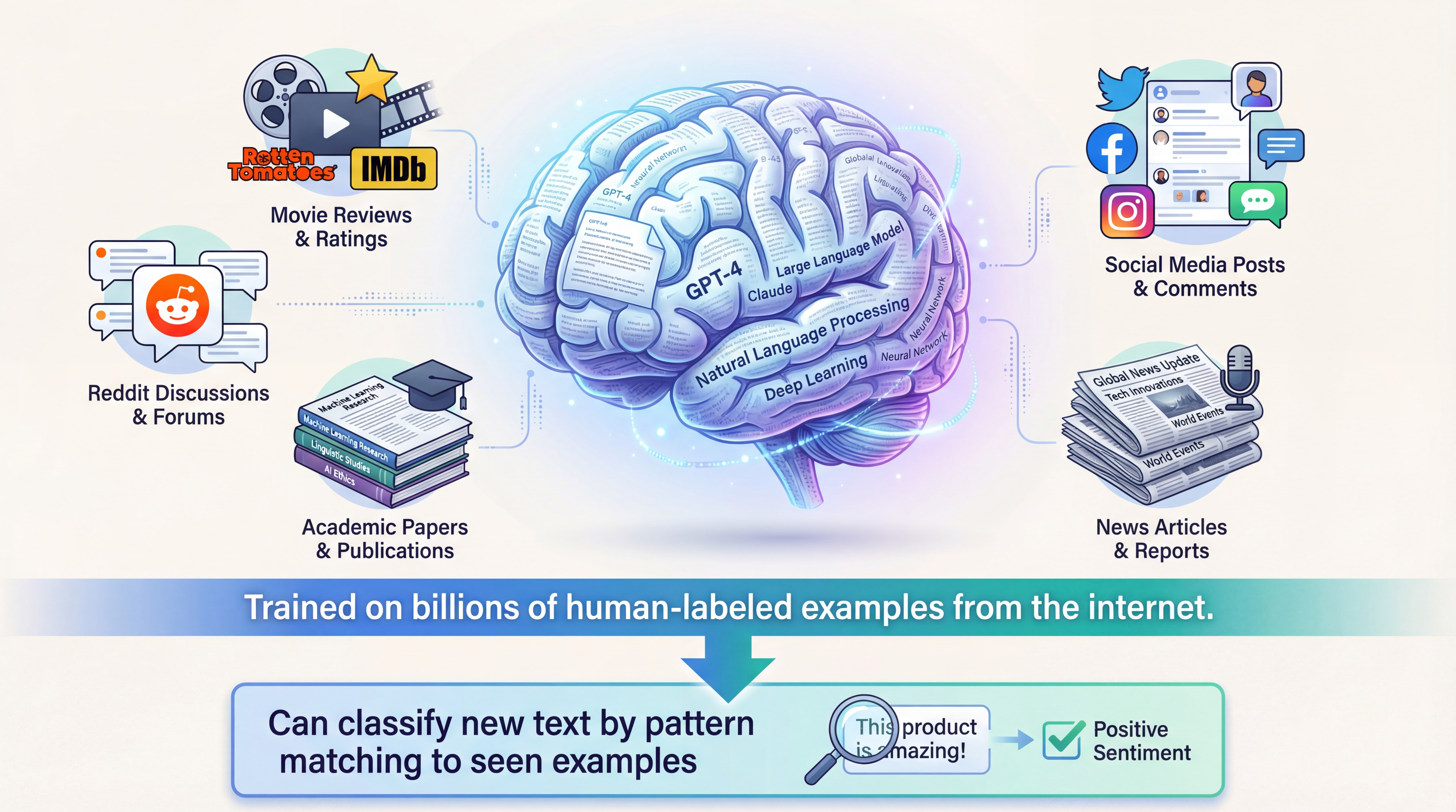
LLMs = Crowdsourced human knowledge, distilled into a model

LLM Labeling: ChatGPT Interface

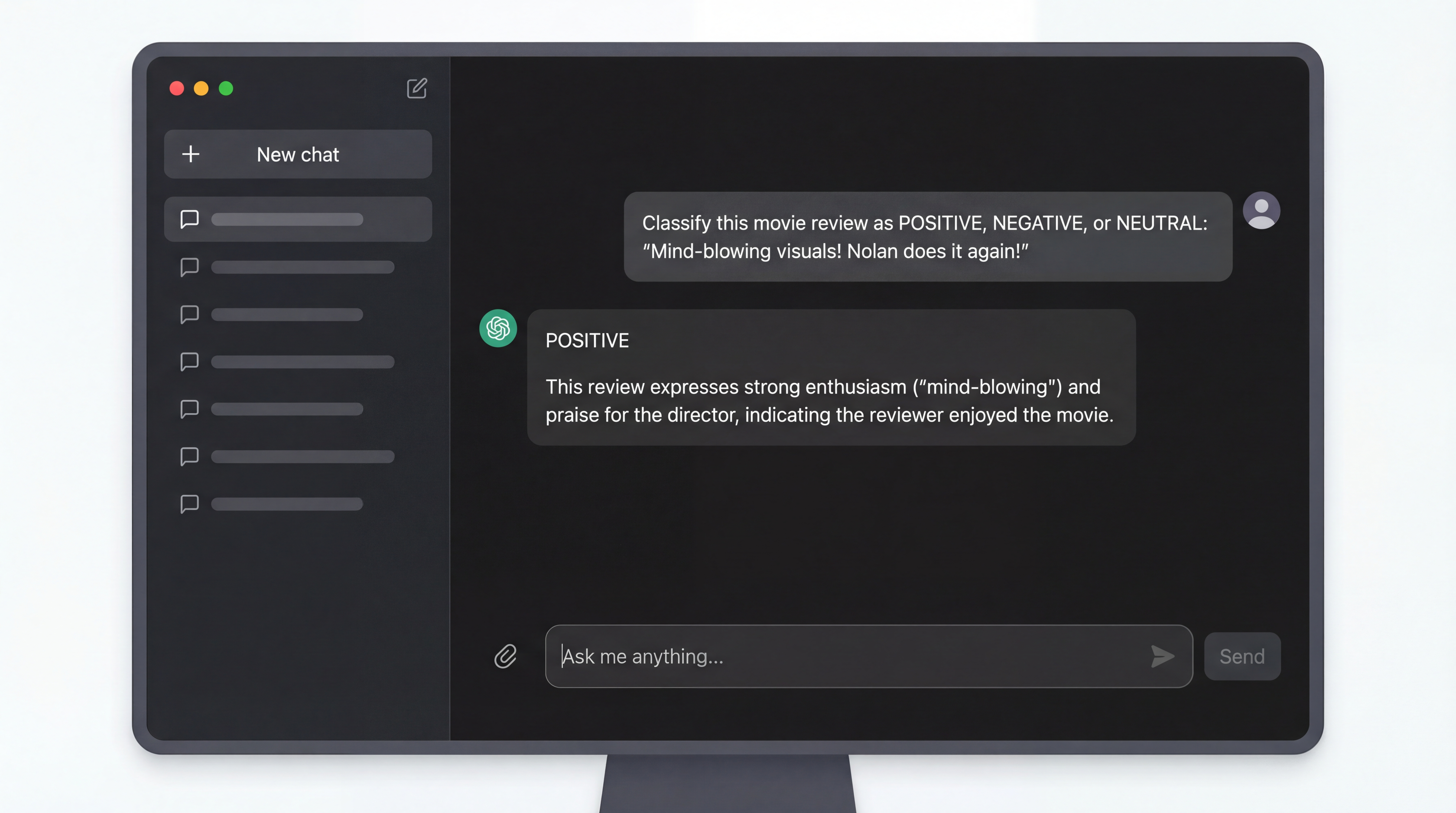
It's this simple! Just ask the LLM to classify text. But how do we scale this to 10,000 reviews?

LLM Labeling: System vs User Messages

messages = [
    {"role": "system", "content": "Classify movie reviews as POSITIVE/NEGATIVE/NEUTRAL"},
    {"role": "user", "content": "Review: 'Mind-blowing visuals! Nolan does it again!'"}
]
# Response: "POSITIVE"

LLM Labeling: API for Scale

from openai import OpenAI
client = OpenAI()

def label_review(review):
    response = client.chat.completions.create(
        model="gpt-4",
        messages=[
            {"role": "system", "content": "Classify as POSITIVE/NEGATIVE/NEUTRAL. Reply with only the label."},
            {"role": "user", "content": f"Review: {review}"}
        ],
        max_tokens=10
    )
    return response.choices[0].message.content.strip()

# Label 1000 reviews
labels = [label_review(r) for r in reviews]

Demo: lecture-demos/week04/llm_labeling.py

Better Prompts = Better Labels

prompt = """Examples:
"Loved it!" → POSITIVE
"Terrible" → NEGATIVE

Now classify: "The movie was okay I guess"
Label:"""

Few-shot examples can improve accuracy by 10-20%!

LLM Labeling Quality Control

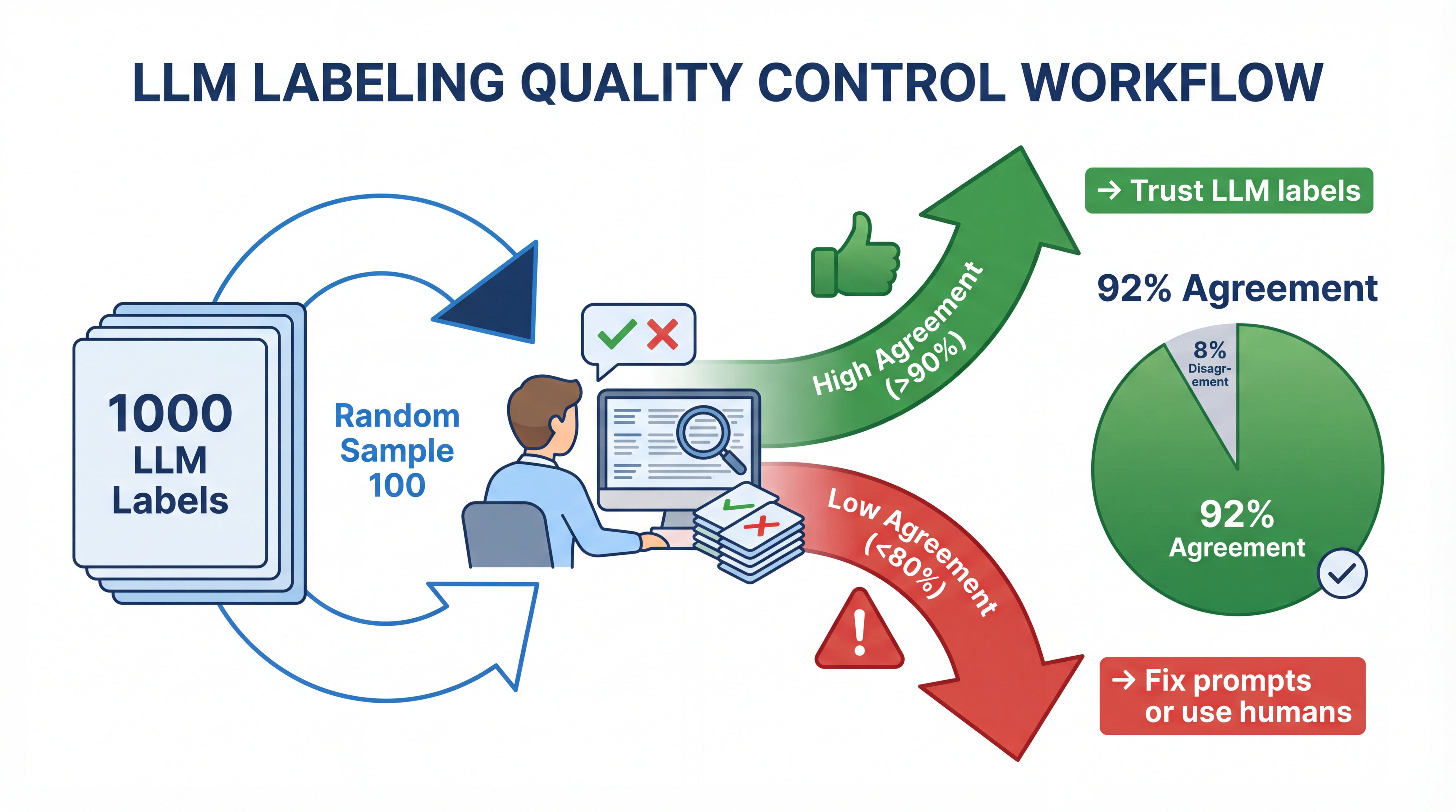
Always validate! Sample 50-100 labels and check human-LLM agreement before trusting the full batch.

When LLMs Struggle

1. Subjective Tasks

"This movie is so bad it's good"
LLM: NEGATIVE (wrong - it's ironic praise!)

2. Domain-Specific Knowledge

"The mise-en-scene was pedestrian but the diegetic sound..."
LLM: ? (needs film theory knowledge)

3. Nuanced Categories

5-point scale: Very Negative, Negative, Neutral, Positive, Very Positive
LLM accuracy drops significantly with more categories

4. Ambiguous Guidelines

What exactly counts as "slightly negative"?

Hybrid Approach: LLM + Human

def hybrid_labeling(texts, confidence_threshold=0.8):
    llm_labels = []
    human_queue = []

    for i, text in enumerate(texts):
        label, confidence = label_with_confidence(text)

        if confidence >= confidence_threshold:
            llm_labels.append((i, label, "llm"))
        else:
            human_queue.append(i)

    print(f"LLM labeled: {len(llm_labels)}")
    print(f"Need human: {len(human_queue)}")

    # Send human_queue to annotation platform
    return llm_labels, human_queue

Use LLMs for easy examples, humans for hard ones!

LLM Labeling: Cost Comparison

Sweet spot: GPT-3.5/Claude Haiku for first pass, humans for validation

Sources of Label Noise

Real-world datasets often have 5-20% label noise!

Detecting Label Errors with Cleanlab

Idea: Train model → find where model strongly disagrees with label

Review	Given Label	Model says	Suspicious?
"Loved it!"	POS	95% POS	No
"Not good at all"	POS	92% NEG	Yes!
"Meh, it was fine"	NEG	60% NEG	No

from cleanlab import Datalab
lab = Datalab(data={"X": X, "y": y}, label_name="y")
lab.find_issues(pred_probs=model.predict_proba(X))
mislabeled = lab.get_issues()[lab.get_issues()['is_label_issue']].index

Notebook: lecture-demos/week04/cleanlab_noisy_labels.ipynb

What to Do With Noisy Labels?

Rule of thumb:

• <5% noise → probably fine, ignore it
• 5-15% noise → use cleanlab to remove/fix
• >15% noise → fix your labeling process!

Decision Tree: Which Technique?

Quick decision guide:

Cost-Benefit Analysis

Typical savings: 5-20x cost reduction with hybrid approach

Key Takeaways

1. Active Learning - Let model pick what to label (2-10x savings)

2. Weak Supervision - Write labeling functions (10-100x savings)

3. LLM Labeling - Use GPT/Claude as annotators (10-50x cost reduction)

4. Noisy Labels - Detect and handle with cleanlab

5. Combine approaches - Hybrid pipelines give best results

6. Quality matters - Validate with human spot-checks

7. Tools exist - modAL, Snorkel, cleanlab, OpenAI API

This Week's Lab

Hands-on Practice:

1. Active Learning from scratch

   • Implement uncertainty sampling
   • Compare to random sampling
   • Visualize learning curves

2. Weak Supervision with Snorkel

   • Write labeling functions
   • Train label model
   • Analyze LF quality

3. LLM Labeling

   • Prompt engineering for annotation
   • Compare GPT-3.5 vs GPT-4 quality
   • Calculate cost savings

Lab Setup Preview

# Install required packages
pip install snorkel
pip install cleanlab
pip install openai scikit-learn

# Verify installations
python -c "import snorkel; print('Snorkel OK')"
python -c "import cleanlab; print('cleanlab OK')"
python -c "import sklearn; print('sklearn OK')"

You'll implement a complete labeling optimization pipeline!

Next Week Preview

Week 5: Data Augmentation

• Why augmentation improves models
• Text augmentation techniques
• Image augmentation with Albumentations
• Audio and video augmentation
• When (not) to augment

More data from existing data - without labeling!

Resources

Libraries:

• modAL: https://modal-python.readthedocs.io/
• Snorkel: https://snorkel.ai/
• cleanlab: https://cleanlab.ai/
• OpenAI API: https://platform.openai.com/

Papers:

• "Data Programming" (Snorkel paper)
• "Confident Learning" (cleanlab paper)

Reading:

• Snorkel tutorials: https://www.snorkel.org/use-cases/