What Is a Distribution?
Think of
| Example | Distribution |
Samples |
|---|---|---|
| Email spam detection | All emails ever sent + will be sent | The 1000 emails in your dataset |
| Medical diagnosis | All patients with this condition | The 200 patients in your study |
| Stock prediction | All trading days past and future | The 5 years of historical data |
Your dataset is a tiny window into a much larger reality.
The question: can we learn something from this window that applies to the full distribution?
The i.i.d. Assumption
We assume our data points are i.i.d.: independent and identically distributed.
Identically distributed: Every data point comes from the same distribution
- Monday's emails and Friday's emails follow the same pattern
- Patient 1 and Patient 100 are drawn from the same population
Independent: Knowing one data point tells you nothing about another.
- Seeing one email doesn't change the probability of the next email
- One patient's diagnosis doesn't affect another's
i.i.d. in Code: Sampling from a Distribution
import torch

# The "true" distribution (unknown in real life, we define it here)
D = torch.distributions.Normal(loc=5.0, std=2.0)

# Draw i.i.d. samples — each draw is independent, same distribution
sample1 = D.sample((100,))  # 100 training samples
sample2 = D.sample((50,))   # 50 test samples

print(f"Training mean: {sample1.mean():.2f}")  # ≈ 5.0
print(f"Test mean:     {sample2.mean():.2f}")  # ≈ 5.0
Both sets are drawn from the same
Notebook Section 2: See the i.i.d. demo with PyTorch distributions.
When i.i.d. Breaks Down
| Violation | Example | Consequence |
|---|---|---|
| Not identical | Train on summer, test on winter | Model fails on new season |
| Not independent | Time series: today depends on yesterday | Random splits leak future info |
| Distribution shift | Train in lab, deploy in the wild | Model accuracy drops |
Most of this lecture assumes i.i.d. holds. When it doesn't (time series, grouped data), we need special CV strategies — covered in Section 5.
What We Want: Generalization Error
Given samples from
We want to know: how well will
This is the expected loss on a randomly drawn new data point — the generalization error.
Breaking Down the Math
| Symbol | Meaning |
|---|---|
| Our trained model's prediction for input |
|
| The true label for that input | |
| Loss function: how wrong is the prediction? (e.g., 0-1 loss, MSE) | |
| A new data point drawn from the real-world distribution |
|
| Expected value — average over all possible new data points |
In plain English: "On average, how much error will our model make on data it has never seen?"
From Theory to Practice
Theory (impossible): Average loss over ALL possible data from
We can't compute this — we'd need infinite data.
Practice (what we do): Average loss over a finite held-out set
The entire lecture is about making
Section 2: Train/Test Split
The simplest evaluation strategy
Our Dataset: Study Hours vs Exam Pass/Fail
import numpy as np

np.random.seed(42)
hours = np.random.uniform(1, 10, 100)
noise = np.random.normal(0, 1, 100)
pass_fail = (hours + noise > 5).astype(int)

X = hours.reshape(-1, 1)
y = pass_fail
A dataset students can relate to — study hours predict exam outcome.
Notebook Section 1: Build this dataset, visualize the scatter plot, see the decision boundary.
Why Not Evaluate on Training Data?
dt = DecisionTreeClassifier()  # no depth limit!
dt.fit(X, y)
print(f"Training accuracy: {dt.score(X, y):.3f}")  # 1.000
100% accuracy! Should we celebrate?
No. The model memorized every training example. It's like a student who memorizes all practice questions word-for-word:
Practice test:  100%  ← memorization
Actual exam:     60%  ← can't generalize
Training accuracy measures memorization, not generalization.
Notebook Section 3: See this yourself — unlimited depth tree gets 100% train but much lower test.
The Basic Idea: Hold Out Test Data
Divide the dataset into two non-overlapping parts:
X_train, X_test, y_train, y_test = train_test_split(
    X, y, test_size=0.2, random_state=42)

model = DecisionTreeClassifier(max_depth=3)
model.fit(X_train, y_train)

print(f"Train accuracy: {model.score(X_train, y_train):.3f}")
print(f"Test accuracy:  {model.score(X_test, y_test):.3f}")
The model trains on 80%, is evaluated on the other 20% it has never seen.
Notebook Section 4: Try different
test_sizevalues andrandom_stateseeds.
Problem: One Split Is Unreliable
for seed in [1, 2, 3, 4, 5]:
    X_tr, X_te, y_tr, y_te = train_test_split(
        X, y, test_size=0.2, random_state=seed)
    model.fit(X_tr, y_tr)
    print(f"Split {seed}: {model.score(X_te, y_te):.0%}")
Split 1 → 82%     Split 4 → 74%
Split 2 → 78%     Split 5 → 84%
Split 3 → 86%
Which is the real accuracy? It depends on which 20 samples ended up in the test set.
Visualizing Split Variance
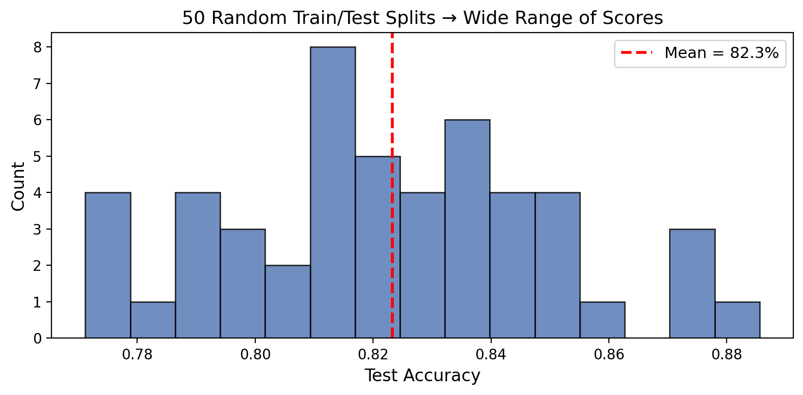
Same model, same data, 50 different accuracy numbers. Range: 10+ percentage points.
One split = one sample from the distribution of possible test sets. Samples have variance.
Notebook Section 5: Run 50 random splits, plot the histogram, compute the std.
Section 3: Model Complexity
We can split data. But which model should we evaluate?
What Is Model Complexity?
Every model has knobs that control how flexible it is:
| Model | Complexity Knob | More complex → |
|---|---|---|
| Polynomial regression | degree |
Higher degree → more wiggly |
| Decision tree | max_depth |
Deeper → more specific rules |
| Neural network | Layers, neurons | More params → more capacity |
| KNN | k (neighbors) |
Fewer neighbors → more flexible |
More complex ≠ better. There's a sweet spot.
Polynomial Fits: Degree 1, 3, and 15
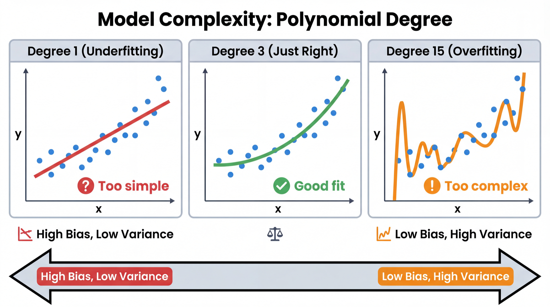
Degree 1: Misses the curve entirely (underfitting)
Degree 3: Captures the pattern, ignores noise (good fit)
Degree 15: Passes through every point — memorizes noise (overfitting)
Polynomial Fits in Numbers
for degree in [1, 3, 15]:
    pipe = Pipeline([
        ('poly', PolynomialFeatures(degree=degree)),
        ('lr', LinearRegression())
    ])
    pipe.fit(X_train, y_train)
    print(f"Degree {degree:2d}: "
          f"Train R²={pipe.score(X_train, y_train):.3f}  "
          f"Test R²={pipe.score(X_test, y_test):.3f}")
Degree  1: Train R²=0.421  Test R²=0.398   ← both low = underfitting
Degree  3: Train R²=0.891  Test R²=0.872   ← both high = good
Degree 15: Train R²=0.999  Test R²=0.214   ← gap = overfitting!
Notebook Section 6: Fit degrees 1-15, plot train vs test R² to see the full curve.
Decision Trees: Same Story
for depth in [1, 4, 20, None]:
    dt = DecisionTreeClassifier(max_depth=depth, random_state=42)
    dt.fit(X_train, y_train)
    print(f"depth={str(depth):>4s}: "
          f"Train={dt.score(X_train, y_train):.3f}  "
          f"Test={dt.score(X_test, y_test):.3f}")
depth=   1: Train=0.731  Test=0.720   ← underfitting
depth=   4: Train=0.862  Test=0.845   ← good
depth=None: Train=1.000  Test=0.762   ← severe overfitting
100% training accuracy is a red flag, not a celebration.
The U-Shaped Curve
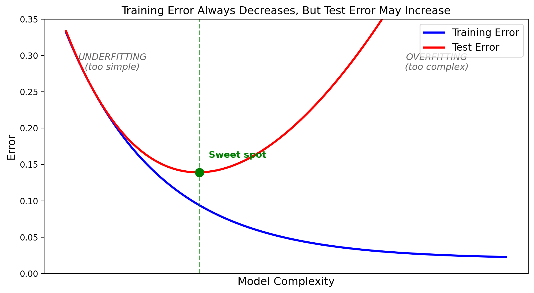
As complexity increases: training error always goes down, but test error goes down then back up. The gap between them = overfitting.
Bias-Variance Tradeoff
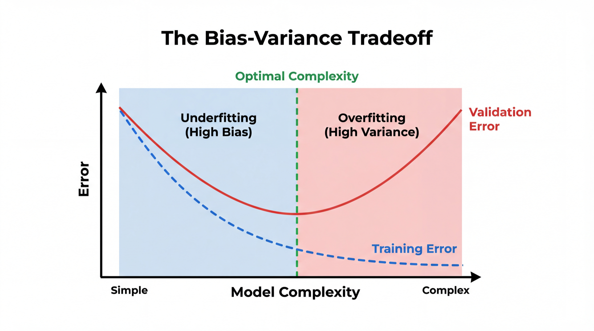
Bias = consistently wrong (model too simple). Like a broken clock.
Variance = inconsistent across datasets (model too complex). Like a nervous student.
The sweet spot minimizes their sum.
Diagnosing and Fixing Your Model
| Train Acc | Test Acc | Gap | Diagnosis | Fix |
|---|---|---|---|---|
| 70% | 68% | 2% | Underfitting | More complex model, more features |
| 85% | 83% | 2% | Good fit | Ship it! |
| 99% | 65% | 34% | Overfitting | Simpler model, more data, regularization |
Rule of thumb: Train-test gap > 10% → you're probably overfitting.
Question: How do we choose the right complexity? We need a validation set.
Notebook Section 6: Experiment with different depths and degrees. Find the sweet spot.
Section 4: The Validation Set
Choosing between models without contaminating the test set
The Problem: Using Test Set for Decisions
You try 100 tree depths and pick the one with the best test score:
depth=1:   test=72%
depth=2:   test=76%
...
depth=47:  test=87%  ← "Best! Let's report this!"
That 87% is optimistically biased. You searched 100 options and picked the luckiest. The model doesn't actually perform that well on new data.
Using the test set for ANY decision contaminates your evaluation.
Solution: Three-Way Split
Training set   (60%) → model learns parameters
Validation set (20%) → choose best hyperparameters
Test set       (20%) → final one-time evaluation
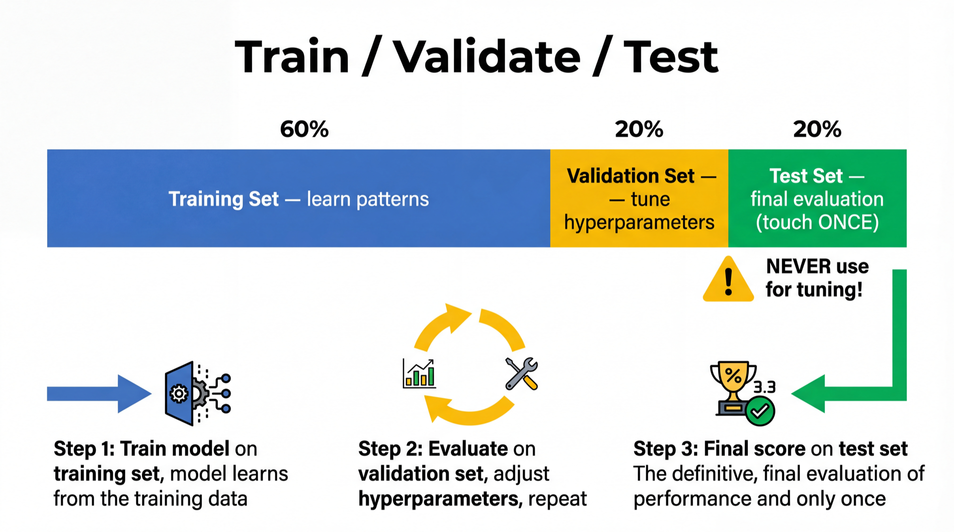
The test set is a sealed envelope. Open it once, at the end.
Three-Way Split in Code
# Two nested splits: first test, then validation
X_trainval, X_test, y_trainval, y_test = train_test_split(
    X, y, test_size=0.2, random_state=42)
X_train, X_val, y_train, y_val = train_test_split(
    X_trainval, y_trainval, test_size=0.25, random_state=42)
# Search hyperparameters on VALIDATION set
best_depth, best_score = None, 0
for depth in [1, 2, 3, 5, 10, 20]:
    dt = DecisionTreeClassifier(max_depth=depth)
    dt.fit(X_train, y_train)
    val_acc = dt.score(X_val, y_val)
    if val_acc > best_score:
        best_depth, best_score = depth, val_acc
Notebook Section 7: Implement three-way split and find the best depth.
Final Evaluation
# Retrain on ALL non-test data (train + validation combined)
final = DecisionTreeClassifier(max_depth=best_depth)
final.fit(X_trainval, y_trainval)

print(f"Final test accuracy: {final.score(X_test, y_test):.3f}")
Key: Retrain on X_trainval — don't waste validation data after you've chosen.
Problem: We're Wasting Data
Train:      600 samples  (60%)
Validation: 200 samples  (20%)  ← only used for selection
Test:       200 samples  (20%)  ← only used once
Only training on 60% of data. With small datasets, this hurts model quality.
Also: the validation score depends on which 200 samples landed in validation. Same variance problem!
Can we do better? Yes — cross-validation.
Section 5: Cross-Validation
Use ALL data for both training and validation
K-Fold Cross-Validation
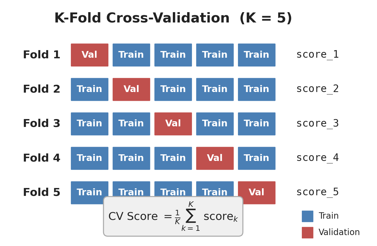
K-Fold: How It Works
- Split data into K equal folds (K=5 is standard)
- For each fold: use it as validation, train on the other K-1
- Average the K scores → CV Score
Every data point is used for validation exactly once and for training K-1 times.
With K=5: each model trains on 80% of data (vs 60% in three-way split).
Implementing K-Fold: Setup
K = 5
indices = np.arange(len(X))
np.random.shuffle(indices)
folds = np.array_split(indices, K)  # 5 roughly equal chunks
folds[0] = [23, 7, 45, 12, ...]   ← validation in round 0
folds[1] = [3, 88, 51, 9, ...]    ← validation in round 1
...
Each fold takes a turn as the validation set.
Implementing K-Fold: The Loop
scores = []
for k in range(K):
    val_idx = folds[k]
    train_idx = np.concatenate(
        [folds[j] for j in range(K) if j != k])
    model = DecisionTreeClassifier(max_depth=5)
    model.fit(X[train_idx], y[train_idx])
    scores.append(model.score(X[val_idx], y[val_idx]))

print(f"Mean: {np.mean(scores):.3f} ± {np.std(scores):.3f}")
Notebook Section 8: Implement this yourself. Verify it matches sklearn.
sklearn: Two Lines
from sklearn.model_selection import cross_val_score

model = DecisionTreeClassifier(max_depth=5)
scores = cross_val_score(model, X, y, cv=5)

print(f"Fold scores: {scores}")
print(f"Mean: {scores.mean():.3f} ± {scores.std():.3f}")
Fold scores: [0.82, 0.85, 0.80, 0.84, 0.83]
Mean: 0.828 ± 0.017
Report as: "82.8% ± 1.7% accuracy (5-fold CV)"
Notebook Section 9: Compare manual CV vs
cross_val_score.
Why CV Is Better
Single split:  82%     (but could be 74% or 88%)
5-fold CV:     82.8%   ± 1.7% (stable + uncertainty!)
- More stable — averaged over K splits
- Uncertainty estimate — the ± std tells you how trustworthy the score is
- Better data usage — every sample used for both training and validation
Choosing K
| K | Train % | Tradeoff |
|---|---|---|
| 2 | 50% | Fast, but each fold only trains on half the data |
| 5 | 80% | Standard default. Good balance. |
| 10 | 90% | More data per fold, but 2× slower than K=5 |
| N (LOO) | N-1 | Uses maximum data, but very slow for large N |
Rule of thumb: Use K=5 unless you have a good reason not to.
Stratified K-Fold: The Problem
If your dataset is 70% class A, 30% class B:
Random Fold 1:  [A A A A A A A A A B]  → 90% A, 10% B  ← unrepresentative!
Random Fold 2:  [A B B B B A A A A A]  → 60% A, 40% B  ← also wrong!
Some folds might have almost no minority class. The model trained on that fold sees a distorted world.
Stratified K-Fold: The Idea
Stratified K-Fold ensures every fold has the same class ratio as the full dataset.

How? Separate samples by class, then deal them round-robin into folds.
Stratified K-Fold: From Scratch (Diagram)
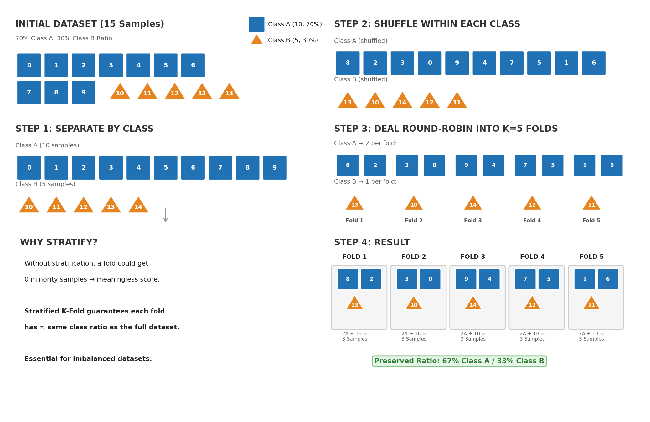
Key idea: Separate by class → shuffle within each class → deal round-robin into K folds.
Each fold preserves the original class ratio.
Stratified K-Fold: From Scratch (Code)
def stratified_kfold(y, K, seed=42):
    np.random.seed(seed)
    classes = np.unique(y)
    folds = [[] for _ in range(K)]
    for cls in classes:
        cls_indices = np.where(y == cls)[0]
        np.random.shuffle(cls_indices)
        # Deal indices round-robin to folds
        for i, idx in enumerate(cls_indices):
            folds[i % K].append(idx)
    return [np.array(f) for f in folds]

folds = stratified_kfold(y, K=5)
# Check: each fold has same class ratio
for k, f in enumerate(folds):
    print(f"Fold {k}: {y[f].mean():.1%} positive")
Notebook Section 10: Implement stratified K-Fold from scratch, compare class ratios.
Stratified K-Fold: The Punchline
All that from-scratch logic? sklearn does it in one argument:
# Option 1: Explicit
skf = StratifiedKFold(n_splits=5, shuffle=True, random_state=42)
scores = cross_val_score(model, X, y, cv=skf)

# Option 2: It's already the default for classifiers!
scores = cross_val_score(model, X, y, cv=5)  # stratified automatically
Why did we implement it from scratch? So you understand what stratification does and why it matters — not just how to call it.
Time Series: When i.i.d. Breaks
With time series data, the i.i.d. assumption doesn't hold — tomorrow depends on today. Random splits let the model peek at the future:
BAD (random split):
  Train: [Jan, Mar, Jun, Aug]  Test: [Feb, May]  ← model sees the future!

GOOD (temporal split):
  Train: [Jan, Feb, Mar]  Test: [Apr]  ← always past → future
Time Series Split
from sklearn.model_selection import TimeSeriesSplit

tscv = TimeSeriesSplit(n_splits=5)
for train_idx, test_idx in tscv.split(X_stock):
    print(f"Train: [{train_idx[0]}..{train_idx[-1]}] "
          f"→ Test: [{test_idx[0]}..{test_idx[-1]}]")
Train: [0..38]    → Test: [39..65]
Train: [0..65]    → Test: [66..98]
Train: [0..98]    → Test: [99..131]
Train: [0..131]   → Test: [132..164]
Train: [0..164]   → Test: [165..197]
Training window grows. Always: past predicts future.
Time Series Example: Stock Prices
# Simple stock prediction: will tomorrow be up or down?
np.random.seed(42)
prices = np.cumsum(np.random.randn(200)) + 100  # random walk
returns = np.diff(prices)
X_stock = returns[:-1].reshape(-1, 1)  # today's return
y_stock = (returns[1:] > 0).astype(int)  # tomorrow up?

# WRONG: random split
wrong_cv = cross_val_score(model, X_stock, y_stock, cv=5)

# RIGHT: time series split
right_cv = cross_val_score(model, X_stock, y_stock,
                           cv=TimeSeriesSplit(n_splits=5))
print(f"Random CV:      {wrong_cv.mean():.3f}  ← optimistic!")
print(f"TimeSeries CV:  {right_cv.mean():.3f}  ← realistic")
Notebook Section 10: Run both CV types on stock data and see the difference.
Group K-Fold: When Samples Are Not Independent
Multiple data points from the same source violate independence:
| Domain | Group | Problem if split randomly |
|---|---|---|
| Medical imaging | Patient ID | Model recognizes the patient, not the disease |
| NLP | Document ID | Model memorizes writing style |
| Audio | Speaker ID | Model recognizes the voice, not the word |
Group K-Fold: How It Works
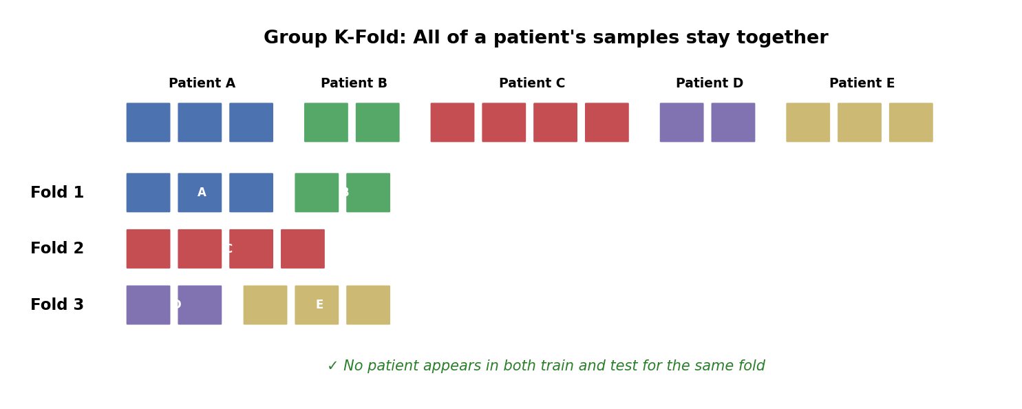
All samples from a patient go into the same fold. When that fold is the test set, the model has never seen that patient.
Group K-Fold in Code
from sklearn.model_selection import GroupKFold

# Each patient has multiple scans
patient_ids = np.array([1,1,1, 2,2, 3,3,3,3, 4,4, 5,5,5])

gkf = GroupKFold(n_splits=5)
for train_idx, test_idx in gkf.split(X, y, groups=patient_ids):
    train_patients = set(patient_ids[train_idx])
    test_patients = set(patient_ids[test_idx])
    print(f"Train patients: {train_patients}, "
          f"Test patients: {test_patients}")
    # No patient appears in both!
All of a patient's data stays together. No leakage across groups.
Notebook Section 10: Implement GroupKFold with a patient dataset.
Leave-One-Subject-Out (LOSO)
A special case of Group K-Fold where K = number of subjects.
from sklearn.model_selection import LeaveOneGroupOut

logo = LeaveOneGroupOut()
for train_idx, test_idx in logo.split(X, y, groups=patient_ids):
    # Test on ONE patient, train on all others
    test_patient = set(patient_ids[test_idx])
    print(f"Test patient: {test_patient}")
Very common in medical/wearable data: train on 9 patients, test on the 10th, rotate.
Gives the most thorough evaluation but expensive if you have many subjects.
CV Variant Cheat Sheet
| Your Data | Use | Why |
|---|---|---|
| Classification (default) | StratifiedKFold |
Maintains class balance |
| Time series | TimeSeriesSplit |
Respects temporal order |
| Grouped samples | GroupKFold |
Prevents group leakage |
| Medical/wearable | LeaveOneGroupOut |
LOSO — test on each subject |
| Tiny dataset (< 50) | LeaveOneOut |
Maximum data for training |
| Everything else | KFold |
Simple, effective |
Section 6: Putting It All Together
Comparing models with cross-validation
The Gold Standard: Compare Model Families with CV
You have data and several candidate model types. Which family works best?
(Not tuning hyperparameters — that's Week 8.)
Step 1:  Pick candidate model families
         (e.g., Decision Tree vs Random Forest vs SVM).

Step 2:  Run K-fold CV on each (default hyperparameters).
         (Use StratifiedKFold for classification)

Step 3:  Compare CV scores (mean ± std).
         Pick the best family.

Step 4:  Retrain the winner on ALL data. Deploy.
That's it. CV tells you which model type fits your problem. Hyperparameter tuning (Week 8) squeezes more performance later.
Comparing Models in Code
from sklearn.model_selection import cross_val_score

candidates = [
    ("Tree(d=3)",  DecisionTreeClassifier(max_depth=3)),
    ("Tree(d=10)", DecisionTreeClassifier(max_depth=10)),
    ("RF(100)",    RandomForestClassifier(n_estimators=100)),
    ("SVM",        SVC()),
]

for name, model in candidates:
    scores = cross_val_score(model, X, y, cv=5)  # stratified by default
    print(f"{name:12s}  CV = {scores.mean():.3f} ± {scores.std():.3f}")
Tree(d=3)     CV = 0.788 ± 0.024
Tree(d=10)    CV = 0.762 ± 0.031   ← overfitting (high variance)
RF(100)       CV = 0.841 ± 0.018   ← winner!
SVM           CV = 0.822 ± 0.021
After Choosing: Retrain on All Data
# Best model chosen by CV: Random Forest
best = RandomForestClassifier(n_estimators=100)
best.fit(X, y)  # retrain on ALL data — maximize what the model learns
Why retrain? During CV, each fold only trained on 80% of data. Now that we've made our choice, give the model everything.
Notebook Section 11: Compare multiple model families with CV, pick the best, retrain.
Common Mistakes
| Mistake | Why It's Wrong | Fix |
|---|---|---|
| Evaluate on training data | Measures memorization | Use cross-validation |
| Use test set to pick hyperparameters | Contaminates evaluation | Use CV to compare |
| Report best of many random splits | Cherry-picking | Use CV, report mean ± std |
| Shuffle time series | Data leakage | Use TimeSeriesSplit |
| Same patient in train and test | Data leakage | Use GroupKFold |
The Lucky Seed Problem
# "Researcher" tries 1000 random seeds, reports the best one
best_acc = 0
for seed in range(1000):
    X_tr, X_te, y_tr, y_te = train_test_split(
        X, y, test_size=0.2, random_state=seed)
    model.fit(X_tr, y_tr)
    acc = model.score(X_te, y_te)
    if acc > best_acc:
        best_acc, best_seed = acc, seed

print(f"Best accuracy: {best_acc:.1%} (seed={best_seed})")
# Looks great! But it's just the luckiest split.
This is a real problem in ML research.

Fix: Always report mean ± std over multiple seeds or use CV.
Section 7: Bridge to Week 8
What's Next: Week 8
This week: How to evaluate a model correctly.
Next week: How to find the best model automatically.
| Topic | What It Does |
|---|---|
| Grid search | Try all hyperparameter combos (nested for-loops) |
| Random search | Sample combos randomly (often better!) |
| Bayesian optimization | Learn from past results to pick next trial |
| AutoML | Automate the whole model + hyperparameter search |
| Experiment tracking | Log and compare 100+ runs |
All of these use cross-validation internally. Week 7 is the foundation for Week 8.
Summary (1/2)
| Concept | Key Idea |
|---|---|
| Distribution |
Data comes from an unknown distribution; we only see samples |
| i.i.d. | Samples are independent and identically distributed |
| Generalization | We want |
| Train/test split | Never evaluate on training data |
| Split variance | One split is unreliable; scores vary by 10%+ |
| Model complexity | Degree, depth, layers control under/overfitting |
Summary (2/2)
| Concept | Key Idea |
|---|---|
| Bias-variance | Simple → bias; complex → variance; sweet spot in between |
| Validation set | Third split to choose hyperparameters |
| K-fold CV | All data used for training AND validation |
| Stratified CV | Maintain class ratios in each fold |
| Time series CV | Always train on past, predict future |
| Group CV | Keep grouped samples together |
| Model comparison | CV all candidates → pick best → retrain on all data |
Exam Questions (1/4)
Q1: You train a model and get 99% training accuracy and 60% test accuracy. What happened?
Overfitting — the model memorized training data. Fix: reduce complexity, add regularization, or get more data.
Exam Questions (2/4)
Q2: What does i.i.d. mean and why does it matter for evaluation?
Independent and Identically Distributed. Each sample comes from the same distribution D and doesn't depend on others. It matters because our evaluation assumes test data follows the same distribution as training data.
Q3: Why can't you use the test set to pick hyperparameters?
Using the test set for decisions contaminates your final evaluation. The reported score would be optimistically biased.
Exam Questions (3/4)
Q4: You have patient data with multiple scans per patient. Why is standard K-fold wrong?
If the same patient appears in train and test, the model might recognize the patient rather than learn the disease pattern. Use
GroupKFoldwith patient ID as the group.
Q5: You're predicting stock prices. Why can't you use standard K-fold?
Stock prices are time-dependent (not i.i.d.). Random splits let the model see future data. Use
TimeSeriesSplit— always train on past, predict future.
Exam Questions (4/4)
Q6: How do you compare multiple models and pick the best one?
Run K-fold CV on each candidate model. Compare mean ± std of CV scores. Pick the model with the best CV score. Retrain it on all available data.
Q7: Implement stratified K-fold from scratch (pseudocode).
For each class: get indices, shuffle, deal round-robin into K folds. This ensures each fold has the same class ratio as the full dataset.
Questions?
Don't trust a single number. Cross-validate.
Understand your model's complexity knobs.
Compare candidates with CV, pick the best, retrain on all data.
Next week: Hyperparameter Tuning, AutoML & Experiment Tracking