Notation used on this pagesymbols, meanings, shapes
    01

    Optional recap: earlier intuition

    Optional labs, worked examples and reference diagramsOPTIONAL REFERENCE DECKOpen the boxes when you need the details.

    The main 54-slide lecture is complete without this material.

    The main 54-slide lecture is complete without this material.

    The main 54-slide lecture is complete without this material.

    We already know how an encoder builds contextENCODER. Encode the input. DECODER. Predict the next token. ENCODER-DECODER. Generate from a source. . . . . . . . Encoder. . . . . . . one vector per token. labels · retrieval · readouts. . . . . Decoder. next. append → repeat. chat · code · continuation. Encoder. . . . target prefix. source K,V. Decoder. next. source + target prefix. translation · summarizationENCODEREncode the inputDECODERPredict the next tokenENCODER-DECODERGenerate from a sourceEncoderone vector per tokenlabels · retrieval · readoutsDecodernextappend → repeatchat · code · continuationEncodertarget prefixsource K,VDecodernextsource + target prefixtranslation · summarization

    Today we reuse the encoder on the left: image patches become tokens, and the final image representation predicts a label.

    The encoder, shown on the left. The full attention square lets every token read every token. The decoder uses causal attention and repeats next-token prediction. The encoder–decoder adds a source pathway into the target decoder through cross-attention. For ViT, replace text tokens with image patches, then use a classification head.

    Today we reuse the encoder on the left: image patches become tokens, and the final image representation predicts a label.

    Summary diagram reused from Transformers beyond next-token prediction (“Encoder, decoder-only and encoder-decoder models”). The same token rows, attention patterns and source-to-target pathway connect this lecture to that recap.

    A ViT is an encoder over image patchesTEXTCLSRaghavgoestoschoolEncoder blockswhole-input attentionRead final CLS→ classifierIMAGECLSP1P2…P196Encoder blockswhole-input attentionRead final CLS→ classifierSame encoder idea. Different tokens.Blue: vision states Purple: language states Amber: learned CLS / position

    Attention builds context in either sequence. The input representation and the task head determine how we use the encoder.

    The input embedding and task head change. The encoder machinery remains: attention, MLPs, residuals and normalization. Both pictured classifiers read final CLS.

    Attention builds context in either sequence. The input representation and the task head determine how we use the encoder.

    Text looks up a row; an image patch computes oneTEXTIMAGE“bank” → token IDEmbedding tablelook up a learned rowtoken content rowD featuresRGB patch: 16 × 16 × 3flatten → 768 valuesShared Linear(768, D)compute a learned projectionpatch content rowD featuresAdd learned position → send the rows into the encoder

    Both routes produce a row of D features. Text learns a vocabulary table; vision learns a shared pixel projection. Our image checkpoint chooses D = 192.

    No. Its pixel values go through a learned affine layer. Once position is added, the encoder works with feature rows in either case.

    Both routes produce a row of D features. Text learns a vocabulary table; vision learns a shared pixel projection. Our image checkpoint chooses D = 192.

    Section 1 · The image classification taskSECTION01The image classification taskA text encoder built context from supplied tokens.What should a model predict from a photograph?Labeled photosThe image taskUseful clues

    The image classification task

    A text encoder built context from supplied tokens.

    What should a model predict from a photograph?

    Labeled photos → The image task → Useful clues

    Start with the dataset, choose an image label, then ask which parts of the photograph help us decide.

    A dataset pairs each image with its target labels. Here the first line under each photo is its species; the second is its breed. These are six selected examples from the test split, chosen to show variety. We use the photos to motivate classification. The optional training lab uses synthetic stripe images, and our pretrained demonstration predicts ImageNet categories. The lecture does not report training or accuracy on the full Pets dataset. Oxford-IIIT Pet dataset, Parkhi, Vedaldi, Zisserman and Jawahar (2012). Pinned mirror metadata. Photos: CC BY-SA 4.0; original image copyrights retained. Example labels, dimensions and provenance.
    What is in this image?One photograph.One image label.What clues did you use?

    Which parts of the photograph helped you decide?

    In Part I, a prefix led to scores for possible next characters. Here a photograph leads to scores for possible image labels. The input and label vocabulary change; the idea of a classifier remains. This is a real Oxford-IIIT Pet image, newfoundland_31.
    Our task today: classify the whole imageimage summarydogcatclass scores

    For the rest of this lecture, we observe the whole photograph and predict one class label.

    This is supervised image classification. The training pair is an image and its class label. The two-label dog/cat example motivates the task; the later pretrained checkpoint uses 1,000 ImageNet labels. Predicting a future or missing patch would require a different objective.
    Attention: what can the face tell this patch?receiver: dark patchfur, shadow, background?patch numberssource: faceface informationsend cluesRecall Q, K, V from textQ (receiver): what to look forK (source): what can matchV (source): information to sendNext: the image versions, then a numerical example.LOCAL ROLESQ / receiverK / sourceV / message

    Attention uses the same Q, K, V roles as in text.

    Vector we followRole
    Query from the dark receiverWhat to look for
    Key from a source such as the faceWhat can match the query
    Value from that sourceInformation to send

    Receiver: this dark crop is ambiguous.

    Source: a face patch elsewhere in the same image.

    Face information → the dark patch’s numbers. Context arrives; the original pixels stay fixed.

    Next: build the image queries, keys and values, then work through a numerical example.

    Queries and keys determine weights; values supply the information to combine. The dark patch is our receiver, and the face patch is one possible source.

    Our task is still to predict one label for the whole image. We are looking inside that computation at one patch. This is attention, using the query, key and value roles introduced for text. For the receiver we follow its query; for a possible source we follow its key and value. Every patch representation actually produces all three vectors. The short descriptions are intuition for numerical vectors, not literal questions or labels stored in the model. By itself the dark crop could suggest fur, shadow or background. Face information could help later layers interpret it. The small arrows from each photograph to its information box stand for representing pixels as numbers. The long arrow shows the direction of information flow: from a source patch into the receiving patch representation. It does not move the source pixels into the receiver. This is an illustration of useful context, not measured attention. The names describe visual clues for students; they are not labels attached to learned vector coordinates. As with bank reading river in Part II, context can make a local representation more useful. The following image examples explain what the vectors could represent; the worked calculation later shows how to compute the weights and combine the values.
    Should every source contribute equally?receiver: dark patchfur, shadow, background?patch numberssource: faceface informationsource: branchesbranch informationlarger sharesmaller shareIllustrative sharesLOCAL ROLESQ / receiverK / sourceV / message

    The receiver is the same dark patch.

    SourceIllustrative contribution
    Face patchLarger share of the message
    BranchesSmaller share of the message

    Attention learns the weights. These shares illustrate the idea; they are not measured results.

    Here, face clues could help more than branches. Attention weights control how much each source contributes to the message.

    Different source patches can contribute different amounts of information. The thick and thin arrows illustrate a possible preference for face clues when interpreting the dark crop. They are not attention weights measured from this photograph, and the model does not have a rule saying faces always matter more. Learned query and key projections determine weights for the current receiver and input. The weights combine the source value vectors into a message. All image patches, including the receiver itself, can be sources in full self-attention; only two sources are drawn here. We will calculate weights and messages in the worked example after constructing patch rows.
    What changes when the patch gets context?receiver: dark patchsame pixelscurrent patch rowface patchface valuebranchesbranch value× its weight× its weightweighted contextsum values + project+updated patch rowTwo sources shown; all image rows can contribute.LOCAL ROLESQ / receiverK / sourceV / message

    The dark crop’s pixels stay unchanged.

    facebranches
    SourceContribution
    Face patch representationface value × its attention weight
    Branch patch representationbranch value × its attention weight

    Sum the weighted values, then apply the output projection to form the context message. Two sources are shown; all image rows can contribute.

    Current patch row + context message → updated patch row.

    Later layers use the updated rows to predict one label for the whole image.

    The face and branches contribute value vectors. Attention weights mix those vectors, and an output projection forms the message added to the dark patch’s row. The pixels stay fixed.

    This previews the attention update with its residual connection. Attention mixes information from source rows, and the block adds the resulting message (after the attention output projection) to the receiver’s existing row. The photograph remains unchanged. The face and branch crops identify where two source representations came from. Their value vectors are computed from those representations; the photo crops themselves are not added to the receiver. Each source value is multiplied by its attention weight for this dark-patch query, then the weighted values are summed and projected to form the update. The query and source keys determine the weights. Only two sources are drawn to show the route. Full image self-attention can use all image rows, including the receiver itself. The diagram illustrates the computation; it does not claim measured weights or fixed meanings for learned coordinates. We have drawn one receiver; other patch rows can receive their own messages too. The later classification readout produces one label for the image. Training here supplies image labels, not fur or eye labels for individual patches. Next we build the numerical rows from pixels, then return to the exact attention calculation.
    What could a query be in the image?Text · receiverbankImage · receivere_bankW_Qq_banke_darkW_Qq_darkWhich context could help bank?Could this dark texture belong to the animal?LOCAL ROLESQ / receiverK / sourceV / message
    Text receiverImage receiver
    bank row → W_Q → q_bankdark-patch row → W_Q → q_dark
    Seek context for bankSeek context for the dark texture

    The row being updated makes a query. Its learned projection determines what kinds of source information it can match.

    For text, q_bank=e_bank W_Q. For vision, q_dark=e_dark W_Q. The operation has the same role in both models; their trained matrices are separate parameters. The plain-language questions illustrate what a query does. A ViT computes numerical queries from its current rows without a text prompt. In the full pre-normalized block, the projection uses the normalized version of the row. We will return to normalization in the complete-block section.
    What could a key be in the image?Text · sourceriverImage · sourcee_riverW_Kk_rivere_faceW_Kk_faceq_bank · k_river → scoreq_dark · k_face → scoreLOCAL ROLESQ / receiverK / sourceV / message
    Text sourceImage source
    river row → W_K → k_riverface-patch row → W_K → k_face
    q_bank compares with source keysq_dark compares with source keys

    Each source row makes a key. Comparing the receiver’s query with source keys gives the scores used to choose attention weights.

    A key is a learned matching vector made from a source row. The text receiver bank can compare its query with river’s key; the dark image patch can compare its query with the face patch’s key. Other source rows have their own keys as well. Scaled query–key dot products are normalized together across allowed sources to form attention weights. The visual names identify crops for students; the model learns the key coordinates from data.
    What information would a value send?Text · sourceriverImage · sourcee_riverW_Vv_rivere_faceW_Vv_faceweight × v_riverweight × v_faceLOCAL ROLESQ / receiverK / sourceV / message
    TextImage
    river row → W_V → v_riverface-patch row → W_V → v_face
    Sum weighted source valuesSum weighted source values

    Q and K choose the weights. V supplies the information to combine using those weights; the combined message updates the receiving representation.

    The river token and the face patch each make a value vector from their current row, using W_V. The receiver sums weighted values from its allowed sources. The output projection maps that message to the width needed for the residual update. This is the same operation illustrated by the preceding source-to-receiver arrows. The original token or crop stays fixed while its representation gains context. The later worked examples calculate the weights and weighted sums explicitly.
    How can we give this photograph to attention?whole photographnumbers for a patchnumbers for a patchnumbers for a patch⋮one row per patchattentionshare information

    Attention works on rows of numbers. Next, we choose image patches and turn their pixels into those rows.

    We have recalled the text computation, asked for the image counterparts of tokens, embeddings and Q/K/V, and chosen an image-classification target. Now assemble the image path. Text supplied one row per token; our image will supply one row per fixed-size patch. This drawing previews the construction. The next section first chooses the patch grid, then reads the pixels and applies a shared learned projection. Position information comes after that.
    The image classifier, drawn as one encoder pipeline224 × 224 RGBShared patch projection196 rows · 192 features+ learned CLS+ learned positionEncoder× 12Final LayerNormread CLS: 192 featuresLinear class head1,000 class scoresViT: Dosovitskiy et al., 2020 · dimensions shown for our ViT-Tiny checkpoint

    Patches become feature rows. Learned CLS and position prepare the input. Encoder blocks build context; the final CLS feeds the classifier.

    The shared patch projection creates 196 rows. CLS adds row 197; position adds location information without changing the shape.

    Patches become feature rows. Learned CLS and position prepare the input. Encoder blocks build context; the final CLS feeds the classifier.

    Architecture adapted from Dosovitskiy et al., 2020. The original paper figure is retained in the optional reference material below.

    Optional reference and extra examples

    To images: An Image is Worth 16 × 16 Words
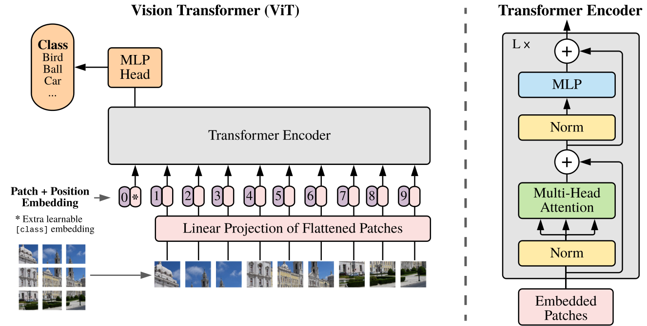
    To images: An Image is Worth 16 × 16 WordsDosovitskiy et al. (2020; ICLR 2021), Figure 1 · arXiv:2010.11929
    Original ViT overview: image patches, linear projection, positions and class token, Transformer encoder, and classification head; an expanded encoder appears on the right

    Image → patches → projected rows + positions + CLS → encoder → image class scores.

    16×16 is the pixel size of one patch. The nine patches drawn in this figure are schematic.

    Dosovitskiy et al. (2020; ICLR 2021), An Image is Worth 16x16 Words: Transformers for Image Recognition at Scale, Figure 1.

    Image patches become tokens. The encoder builds a summary for classification.

    Dosovitskiy et al. (2020; ICLR 2021), An Image is Worth 16x16 Words: Transformers for Image Recognition at Scale, Figure 1. The complete original Figure 1 is reproduced; colored outlines are lecture annotations. The picture at the bottom is cut into patches. A shared linear projection turns each flattened patch into a vector. Add position embeddings and a learned classification token, process the sequence with Transformer encoder blocks, then use the final classification-token representation to score image classes. The right-hand inset opens an encoder block: normalization, multi-head self-attention, an MLP and residual additions. This is an architecture preview; the following photograph walkthrough explains each component when it is needed. The title’s 16×16 refers to a patch’s pixel height and width in a /16 model, not the number of patches or words. The paper figure draws nine patches schematically. Our 224×224 image with 16×16 patches gives a 14×14 grid, or 196 patch tokens. The original figure labels the classifier MLP Head; the saved fine-tuned checkpoint used later in this lecture has a single linear classifier. Open the original figure at full resolution.
    Optional recap and extra examples

    From text: Attention Is All You Need
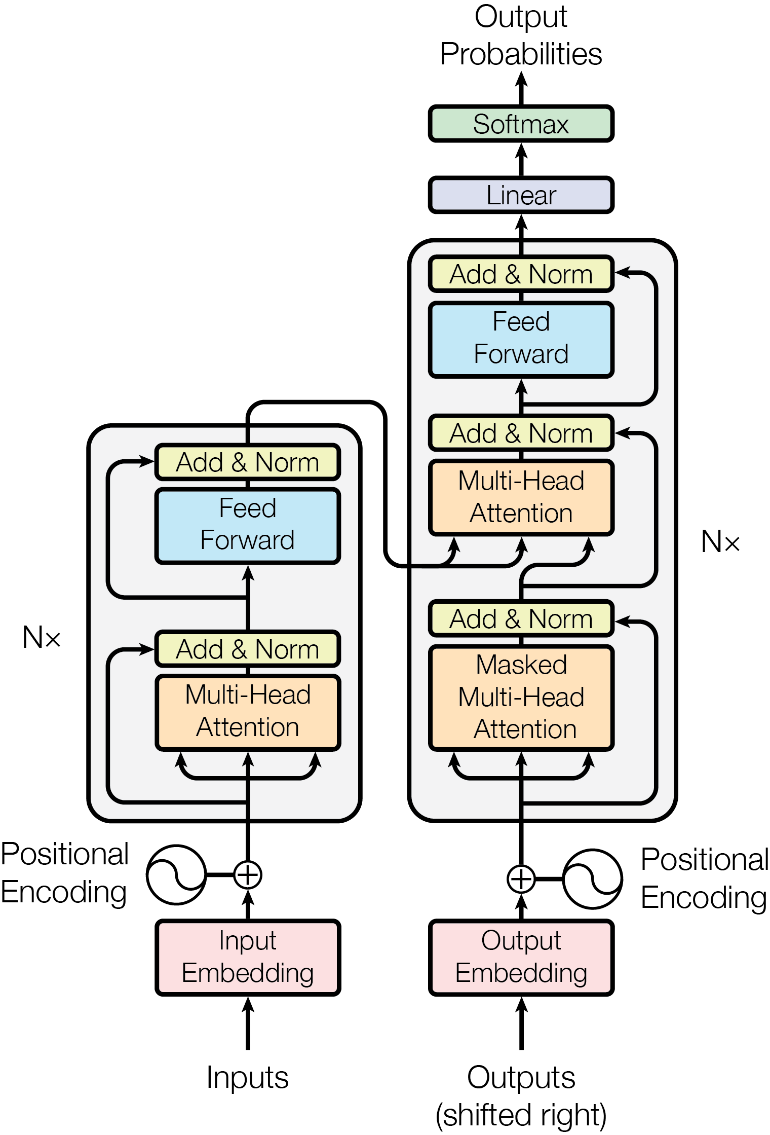
    From text: Attention Is All You Need2017 · a Transformer for translationText tokens → embedding rowsAdd their positions.Encoder: build contextSelf-attention + feed-forward layersDecoder: generate the output textNext: give an encoder image patches.Use its output to classify the image.Vaswani et al. (2017), Figure 1 · arXiv:1706.03762
    Original Transformer figure: encoder on the left, autoregressive decoder on the right

    Follow the encoder: text embeddings + positions → self-attention and feed-forward layers → contextual rows.

    Next: give an encoder image patches and classify the image.

    Vaswani et al. (2017), Attention Is All You Need, Figure 1.

    Follow the encoder: text tokens become rows, then attention gives them context.

    Vaswani et al. (2017), Attention Is All You Need, Figure 1. The authors’ original architecture diagram is reproduced here, with a blue lecture outline added around the encoder. The 2017 paper introduced this encoder–decoder Transformer for sequence transduction, including translation. Both stacks use attention and position-wise feed-forward networks. The encoder reads the available input sequence; the autoregressive decoder uses masked self-attention and cross-attention to the encoder. For this image-classification lecture, the useful connection is the encoder: it updates a sequence of input representations. The next figure replaces text embeddings with projected image patches and adds an image-classification readout. These are related architectures, not identical blocks: the original figure uses normalization after residual addition; the ViT figure places normalization before attention and the MLP. We will unpack our ViT block later. Open the original figure at full resolution.

    How many images and classes are there?

    How many images and classes are there?7,349photographs3,680 train / validation3,669 test2 speciescat or dog37 breedsPersian, Pug, …
    Dataset quantityCount
    Images7,349
    Train / validation3,680
    Test3,669
    Species classes2: cat and dog
    Breed classes37

    Our opening question uses 2 classes: cat or dog. Predicting the breed would use 37 classes.

    The labeled dataset has 7,349 images. The standard training/validation pool contains 3,680 images; the test split contains 3,669. The timm mirror calls the first pool train. Its label_cat_dog field has two species classes, while label has 37 breed classes. We begin with the species question to establish what the input and target mean. The size of the output layer follows the chosen target vocabulary. Oxford-IIIT Pet dataset, Parkhi, Vedaldi, Zisserman and Jawahar (2012). Pinned mirror metadata. Photos: CC BY-SA 4.0; original image copyrights retained. Example labels, dimensions and provenance.

    What shape is one image?

    What shape is one image?Dimensions: height × width × channels334 × 500 × 3resize +center-crop224 × 224 × 3

    Height × width × channels

    Original Newfoundland photograph

    Original: 334 × 500 × 3

    Resize and center-crop ↓

    The exact square model-input crop

    Model input: 224 × 224 × 3 = 150,528 numbers

    Original sizes vary. Our demo uses 224 × 224 pixels, each with red, green and blue values: 150,528 numbers.

    This Newfoundland file is 334 pixels high and 500 wide. The Persian example is 500 high and 375 wide. Both are RGB, so each pixel has three channel values. The diagram uses height × width × channels; PyTorch stores one preprocessed image as [3,224,224], with the same number of entries. For the supplied pretrained checkpoint, preprocessing preserves aspect ratio during resize, takes a 224×224 center crop, and then normalizes the channels. The right-hand image is the saved model-input crop, displayed before normalization. 224×224×3=150,528 scalar inputs. These are pixels, not patch embeddings. Oxford-IIIT Pet dataset, Parkhi, Vedaldi, Zisserman and Jawahar (2012). Pinned mirror metadata. Photos: CC BY-SA 4.0; original image copyrights retained. Example labels, dimensions and provenance.

    Classification: name the animal

    Classification: name the animaldogcat

    Output: one class label for each photograph. Our example labels are dog and cat.

    This is a proposed two-class task, like the email classification task in Part I. The pretrained model later in this lesson has a different label set: 1,000 ImageNet categories. Dog and cat here are human example labels, not outputs from a fitted two-class classifier.

    What were we asking the text model to predict?

    What were we asking the text model to predict?Part I · generate a name, one character at a timea a bwindow + MLPletter scoresnext letterChoose a letter. Append it. Run again.

    Part I · character tokens

    a a b → window embeddings + MLP → character scores → next character.

    Choose one, append it, slide the window and run again.

    A name grows one character at a time. Our fixed-window model scores the possible next characters.

    This recalls Part I’s name-generation model. It looks up embeddings for a fixed window of characters, concatenates them and uses an MLP to score the vocabulary. At generation time, turn scores into probabilities, choose a character and append it; the next call uses the latest window. The vocabulary also includes the boundary token used to end a name. No particular next character or probability is assumed in this diagram. The next slide recalls Part II’s attention model, which uses the updated final token row to predict a word.

    And what were we predicting in the bank example?

    And what were we predicting in the bank example?Part II · continue the river-bank sentenceThe fisherman sat beside the river bankand watchedthe___updated final “the” rowrepresentation after attentionword scoreswaterone possible next wordAppend water, then predict the following word.

    Part II · word tokens

    The fisherman sat beside the river bank and watched the ___

    Updated final the row → vocabulary scores → a possible next word: water.

    Append the chosen word and run again. Bank is an earlier contextual row; the final the row supplies this prediction.

    Here one token is a word. The final “the” row uses the earlier context to predict what comes next; “water” is one plausible continuation.

    The prefix is taken directly from the Part II toy: “The fisherman sat beside the river bank and watched the”. Part II compares this river context with the cheque-and-bank context. Bank has its own contextual representation, but prediction after the full ten-token prefix reads the updated final the row at position 10. The vocabulary head scores all candidate words; softmax turns those scores into probabilities. Water is an illustrative possible choice, not a newly measured model output or the only correct continuation. Appending the chosen word creates a longer prefix for the next generation step. Name generation and sentence continuation both predict the next token, while the token unit and model used in these two lessons differ.

    What changed, and what stayed the same?

    What changed, and what stayed the same?Text generationImage classificationgivenprefix tokenswhole imagepredictnext tokenimage labeluse to predictlast available rowone image summaryloss−log p(next token)−log p(correct class)

    Both models score possible answers. What they observe, summarize and predict differs.

    Both tasks can use the same attention operation and a linear classifier followed by softmax. In the autoregressive setup, each position predicts the next token from its allowed prefix. In the image-classification setup, one image summary predicts the supplied label. Here summary means a vector of numbers used by the classifier. Later we will build that summary and name the two approaches after explaining them. “Text” alone does not imply a causal mask: text encoders can read both directions too.

    Would you recognize this crop on its own?

    What can this patch tell us on its own?We still want one image label. Which clues could help?P10 · one cropNext: attention lets each patch use information from other patches.

    Fur, shadow, or background? Seeing the face elsewhere in the photo helps us interpret this crop.

    The previous slide compared the prediction tasks: next-token prediction uses a text prefix, while image classification predicts one label from the whole image. Now we look inside the image computation. This isolated crop is ambiguous; seeing the face elsewhere in the photo helps us interpret the dark texture. Attention will combine information from other patch representations to update this patch’s representation. The pixels themselves stay fixed. This is the same contextual-representation idea we used for bank in Part II. A patch is a fixed piece of the input, not a word or an object with a ready-made semantic label. The arrow locates the crop in the photograph; it is not a measured attention connection. The following slides unpack how information flows between patches.

    What can we carry over from our text models?

    We already know the operation. What changes?Part IPart IIPart IIIVision Ia a b i driver → bankred / wool → coatrepresentread contextseveral messagesread an imageRepresent → read → update → predict

    We still turn inputs into rows, read useful information, and predict an answer.

    Part I built a character predictor: embeddings, scores, probabilities, loss and learning. Part II gave “bank” a contextual representation. Part III let “coat” read multiple kinds of information. We reuse their row-vector notation, seven colours, and calculation sequence.

    Back to text: what did attention update?

    Back to text: what did attention update?The fisherman sat beside the river bank and watched the …selected tokensembedding + positionread contextupdated rowsriver (6)e₆e₆′bank (7)e₇e₇′the (10)e₁₀e₁₀′Q, K, Vattention+ original rowbank reads positions 1–7; the final the reads positions 1–10.

    The fisherman sat beside the river bank and watched the …

    StepText example
    Tokenbank at position 7
    Initial rowtoken embedding + position
    Read contextQ and K set weights; V supplies information
    Updatee7 + attention update → e7′
    Predict after the full prefixUse the updated final the row, e10′

    Each token starts with an embedding plus position. Attention supplies context; adding its update gives a new representation of the same token.

    Part II: the complete attention diagram and bank in two contexts. The sentence and token embedding are taken from the original text toy. This is a compact redraw of the same text-attention path, with three of the ten rows shown. Every token has an initial embedding plus position, makes query/key/value projections, and receives a context-dependent update. The residual connection adds the projected attention message to the original row. Causal attention lets bank at position 7 read positions 1–7; the last the at position 10 can read all ten observed positions. The contextual bank row helps us understand the mechanism. Next-token prediction after the complete prefix reads the updated final row. During a forward pass these contextual rows change; that is different from updating the embedding-table parameters during training.

    What could be the image equivalent of a token?

    What could be the image equivalent of a token?Text: word tokens in Part IIImage: what should one token be?theriverbankone word → one token rowone patch → one token row
    TextImage
    One token in the word-level toyOne fixed-size image patch
    One row per tokenOne row per patch

    We can use one fixed-size patch as an image token. Each patch gets its own row, just as each text token did.

    Part I used character tokens and the Part II toy used word tokens. ViT uses a regular grid of fixed-size patches. The grid is chosen before the model knows which patches contain the animal. One object can span many patches, and a patch can mix object and background. This slide introduces the correspondence. The next section will calculate the patch count and read the pixel values.

    What could be the image equivalent of an embedding?

    What could be the image equivalent of an embedding?TextImagebankembedding lookup[0.7, 0.7, 0, 0.7]learned pixel projectionone learned patch rowThen add position information to both.
    TextImage
    bank → [0.7, 0.7, 0, 0.7]patch pixels → learned projection → patch row
    Add token positionAdd patch position

    Text uses a learned lookup table. A patch projection produces D coordinates per patch. D is shared across patches and can differ from the number of pixel values.

    Part II: the complete attention diagram and bank in two contexts. The sentence and token embedding are taken from the original text toy. The displayed text vector is the token embedding before position is added. A ViT patch embedding is obtained by flattening the patch pixels and applying a shared learned linear projection, usually with a bias. Both models then add position information to form their initial rows. The embedding widths need not match between the two models. We leave the image row symbolic here because the upcoming slides derive its entries from pixels.

    Could this dark texture belong to the animal?

    Could this dark texture belong to the animal?Same task: one dog/cat label for the whole photograph.receiver P10A possible query:Which patches could connectthis texture to the animal?Possible source clueseye and muzzlemore of the coatq₁₀ = x₁₀ W_Qx₁₀ is the current row for P10.The “question” is a learned vector.

    Receiver P10

    A possible query: Which patches could connect this texture to the animal?

    Source P7: eye and muzzle
    Source P11: more of the coat

    q₁₀ = x₁₀ W_Q. These questions express intuition; the model computes vectors.

    Face and coat clues could help this patch represent part of the animal. The classifier will still predict one label for the whole photo.

    These are human interpretations of possible learned behaviour. No attention head or semantic coordinate is measured on these slides. The classifier receives pixels, and its class-label loss trains the projection matrices. In a full pre-LN block, x denotes a normalized current row. At deeper layers, that row can already contain context from other patches. All three examples use the same W_Q within one head and layer. Different receiver rows can produce different queries. The selected sources illustrate potential context; actual attention compares all allowed keys, including the receiver’s own key. No separate fur, face or branch label is supplied for a patch. Useful contextual features are learned through the whole-image objective.

    Where is the rest of this face?

    Where is the rest of this face?Same task: one dog/cat label for the whole photograph.receiver P7A possible query:Which patches could completethe face around this eye?Possible source cluesother side of the faceneck and coatq₇ = x₇ W_Qx₇ is the current row for P7.The “question” is a learned vector.

    Receiver P7

    A possible query: Which patches could complete the face around this eye?

    Source P6: other side of the face
    Source P11: neck and coat

    q₇ = x₇ W_Q. These questions express intuition; the model computes vectors.

    One patch contains only part of a face. Context from other patches could help its representation describe a larger visual structure.

    These are human interpretations of possible learned behaviour. No attention head or semantic coordinate is measured on these slides. The classifier receives pixels, and its class-label loss trains the projection matrices. In a full pre-LN block, x denotes a normalized current row. At deeper layers, that row can already contain context from other patches. All three examples use the same W_Q within one head and layer. Different receiver rows can produce different queries. The selected sources illustrate potential context; actual attention compares all allowed keys, including the receiver’s own key. No separate fur, face or branch label is supplied for a patch. Useful contextual features are learned through the whole-image objective.

    Where does this branch continue?

    Where does this branch continue?Same task: one dog/cat label for the whole photograph.receiver P4A possible query:Which patches could continuethis branch beyond the crop?Possible source cluesbranch belowbranch to the leftq₄ = x₄ W_Qx₄ is the current row for P4.The “question” is a learned vector.

    Receiver P4

    A possible query: Which patches could continue this branch beyond the crop?

    Source P8: branch below
    Source P3: branch to the left

    q₄ = x₄ W_Q. These questions express intuition; the model computes vectors.

    Background patches can also gather context. A branch representation could use nearby edge continuity; the task still predicts the image label.

    These are human interpretations of possible learned behaviour. No attention head or semantic coordinate is measured on these slides. The classifier receives pixels, and its class-label loss trains the projection matrices. In a full pre-LN block, x denotes a normalized current row. At deeper layers, that row can already contain context from other patches. All three examples use the same W_Q within one head and layer. Different receiver rows can produce different queries. The selected sources illustrate potential context; actual attention compares all allowed keys, including the receiver’s own key. No separate fur, face or branch label is supplied for a patch. Useful contextual features are learned through the whole-image objective.

    What could each source offer for matching?

    What could each source offer for matching?Keep the dark receiver P10: seek clues that connect it to the animal.P7 · eye / muzzleface-like shapeand appearancek₇ = x₇ W_Kcompare q₁₀ with k₇P11 · coatfur-like textureand appearancek₁₁ = x₁₁ W_Kcompare q₁₀ with k₁₁P8 · branchbranch-like edgesand appearancek₈ = x₈ W_Kcompare q₁₀ with k₈

    Receiver: dark patch P10, with query q₁₀.

    P7 · eye / muzzle

    Possible matching features: face-like shape and appearance. k₇ = x₇ W_K.

    P11 · coat

    Possible matching features: fur-like texture and appearance. k₁₁ = x₁₁ W_K.

    P8 · branch

    Possible matching features: branch-like edges and appearance. k₈ = x₈ W_K.

    A different receiver can find different keys relevant. The words describe intuition for numerical vectors.

    A source key can match one query well and another poorly. Comparing this receiver’s query with all source keys sets its attention weights.

    These are human interpretations of possible learned behaviour. No attention head or semantic coordinate is measured on these slides. The classifier receives pixels, and its class-label loss trains the projection matrices. In a full pre-LN block, x denotes a normalized current row. At deeper layers, that row can already contain context from other patches. The crop descriptions give intuition for learned matching features; they are neither key vectors nor fixed semantic labels. Each source makes a key with the same W_K. Relevance belongs to a query–key pair: a source does not have one universal importance score. Scaled dot products followed by softmax choose weights over all allowed sources. The three shown here are a visual subset.

    What information could these values carry?

    What information could these values carry?Use the same source patches. Now ask what information each could send.P7 · eye / muzzleshape around theeye and muzzlev₇ = x₇ W_VP11 · coatcoat textureand colourv₁₁ = x₁₁ W_VP8 · branchbackground edgesand contextv₈ = x₈ W_Vmessage for P10 = a₁₀,₇ v₇ + a₁₀,₁₁ v₁₁ + a₁₀,₈ v₈ + …
    P7 · eye / muzzle

    Possible information to send: shape around the eye and muzzle. v₇ = x₇ W_V.

    P11 · coat

    Possible information to send: coat texture and colour. v₁₁ = x₁₁ W_V.

    P8 · branch

    Possible information to send: background edges and context. v₈ = x₈ W_V.

    Message for P10 = a₁₀,₇ v₇ + a₁₀,₁₁ v₁₁ + a₁₀,₈ v₈ + …

    a₁₀,₇ is the weight for P10 reading P7. Other source values also contribute. Every receiver uses its own weights.

    Each source supplies one value vector. Different receivers mix these values with different weights. Here a₁₀,₇ is the weight for P10 reading P7.

    These are human interpretations of possible learned behaviour. No attention head or semantic coordinate is measured on these slides. The classifier receives pixels, and its class-label loss trains the projection matrices. In a full pre-LN block, x denotes a normalized current row. At deeper layers, that row can already contain context from other patches. The descriptions suggest possible visual information carried by learned features. They are not measured meanings of particular coordinates. Within a head and layer, a source has one value vector shared by all receivers; each receiver can assign a different weight to it. The sum includes every allowed source, including self and CLS where present. It produces a vector that contributes to the receiving row update. This operation neither pastes pixels nor directly chooses the dog/cat label. The classifier later reads the image summary. The dog walkthrough later draws the full Q/K/V matrices and calculates a measured CLS message.

    What is the “next token” for this image?

    What is the “next token” for this image?Text generationImage classificationThe fisherman sat beside theriver bank and watched the ___updated final token rowvocabulary scoresnext token: water, boats, …one image summaryclass scoresimage label: dog or cat
    Text generationImage classification
    Prefix tokensWhole image
    Updated final token rowOne image summary
    Vocabulary scores → next tokenClass scores → image label

    Here the target is an image label. We reuse attention to build representations; our classification task changes what we read out and predict.

    There is no next-token target in this image-classification task. The observed image leads to scores over the class vocabulary. For the text prefix, the updated final the row leads to scores over possible next words; bank’s internal row is not the final prediction row. Both models score possible answers, but the inputs, readout and training targets differ. Image captioning would bring back next-token prediction, conditioned on the image and preceding generated words. Now we have the correspondences. The next drawing assembles the image path, and the following section calculates the patch embeddings.
    02

    Opening the patch-projection box

    Section 2 · From pixels to patch embeddingsSECTION02From pixels to patch embeddingsAttention updates a row of numbers for each token.How do we make those rows from an image?RGB pixelsShared linear layerPatch embeddings

    From pixels to patch embeddings

    Attention updates a row of numbers for each token.

    How do we make those rows from an image?

    RGB pixels → Shared linear layer → Patch embeddings

    Read one small patch, calculate its embedding, then scale the same operation to a real photograph.

    The whole route: photograph to predictionImageonephotographHEREPatchessmallimage cropsHEREProjectionpixels intofeaturesHEREPrepare rowslocation +summaryAttentionshareinformationMLPtransformfeaturesRead summaryone imagevectorClass scoresscore eachimage classInside one blocksoftmax → labelFirst: make the input rowspixels → patch featuresThen: build contextpatches share informationFinally: make a predictionimage summary → labelThe photograph stays fixed. The rows of features change as we follow the arrows.
    1. Image
    2. Patches
    3. Projection
    4. Prepare rows
    5. Attention
    6. MLP
    7. Read summary
    8. Class scores

    Make patch features and prepare the rows. Inside a block, attention shares information and the MLP transforms each row.

    Read one image summary and score the classes. We will open each box as we reach it.

    First turn pixels into patch features. Prepare those rows, let them exchange information, then read one image summary to score the classes. We will open each box as we reach it.

    This map describes the actual ViT-Tiny checkpoint used for the dog photograph. It has D=192, three heads of width 64, 12 blocks and 1,000 ImageNet outputs. CLS means classification token. It is a learned extra input row; its final contextual representation is used to classify the image. The top route is reused on the detailed slides, with the current operation highlighted. The MLP hidden width of 768 happens to equal the patch pixel count; these are separate choices. This is a pre-LayerNorm architecture, so normalization precedes each branch. Both attention and the MLP have residual additions. Original ViT paper. Measured full-model trace · Reproduce every operation.
    Cut on a grid; keep the pieces identifiableP6P7P10P11

    The grid cuts through the photograph before the model knows where the dog is.

    This drawing uses a 4×4 grid so the crops remain large. The real model used at the end takes a 224×224 image and uses 16×16-pixel patches, giving a 14×14 grid. Patch boundaries are chosen before recognition.
    Read the RGB values of each pixelABCD2 × 2 × 3pixelRGBA100B010C001D1114 pixels × 3 channels = 12 values
    ABCD
    PixelRGB / 255
    A[1, 0, 0]
    B[0, 1, 0]
    C[0, 0, 1]
    D[1, 1, 1]

    For this calculation, divide RGB values by 255. Read A, B, C, D: top-left, top-right, bottom-left, bottom-right.

    This small color patch is an illustrative input. A, B, C and D label pixel positions within one patch, not image tokens. Each pixel contributes three channel values. We scale 8-bit values by 255 here; the real pretrained model uses its supplied channel normalization. All inputs, weights and verified outputs.
    Flatten one channel at a time: R, then G, then B4 pixels × 3 channels = 12 valuesABCDone RGB patchR valuesA.R11B.R02C.R03D.R14G valuesA.G05B.G16C.G07D.G18B valuesA.B09B.B010C.B111D.B112A → B → C → D inside each channelOne row x₁: inputs and weights use this same order.
    Channel groupEntries
    R[1, 0, 0, 1]
    G[0, 1, 0, 1]
    B[0, 0, 1, 1]

    x₁ = [1, 0, 0, 1, 0, 1, 0, 1, 0, 0, 1, 1]

    Shape: (1, 12).

    We use all R values, then G, then B: 12 values for this patch. Pixel-by-pixel RGB also works if the weight columns follow that order. Our PyTorch code uses the channel-first order.

    We use channel-major RGB throughout: R_A, R_B, R_C, R_D, G_A, G_B, G_C, G_D, B_A, B_B, B_C, B_D. The row has shape (1,12). Flattening rearranges values and learns no parameters. The weights use this same ordering, matching F.unfold and Conv2d weight.flatten(1). Pixel-first ordering would be A.R, A.G, A.B, B.R, B.G, B.B, C.R, C.G, C.B, D.R, D.G, D.B. Both contain the same 12 values. Neither order is intrinsically more expressive: permuting the input entries and the matching Linear.weight columns preserves every weighted sum. Changing only the input order while keeping trained weights fixed generally changes the result. We choose channel-first throughout to match the implementation. All inputs, weights and verified outputs.
    Do we apply an activation after the patch layer?Patch embedding · at the image input12 pixel valuesnn.Linear(12, 2)2 coordinatesc₁ = x₁W + b. Bias makes this affine; no ReLU or GELU follows.Later, after attention · the block MLPone rowLinear(D, H)GELULinear(H, D)D featuresH featuresH featuresD features

    At the image input: 12 pixel values → nn.Linear(12, 2) → 2 embedding coordinates.

    c₁ = x₁W + b. This affine map has no ReLU or GELU afterward.

    Later, after attention: the block MLP uses Linear(D, H) → GELU → Linear(H, D).

    Feature widths: D → H → H → D. D is the embedding width; H is the hidden width.

    Our patch embedding uses one affine layer. The later block MLP puts GELU between two linear layers. D is the embedding width; H is the MLP’s hidden width.

    In this lecture’s patch layer, cᵢ=xᵢW+b is the complete content projection: no activation is applied to cᵢ. With a bias, this is mathematically an affine transformation; the library calls the layer Linear. The content embedding then receives position information before the Transformer blocks. After attention in our pre-LN block, a normalized current row enters Linear(D,H), GELU, and Linear(H,D); the output participates in a residual addition. This diagram isolates the MLP branch. Our real-image checkpoint uses D=192 and H=768; the RGB hand calculation chooses D=2. The full Transformer also includes operations such as attention softmax and LayerNorm; GELU is the activation inside its MLP. Adding an activation to the patch projection would define a different input module. PyTorch Linear · The lecture’s executable model.
    What does “projection” mean here?Input: x₁Output: c₁12 valuesnn.Linear(12, 2)2 coordinates(1, 12)(1, 2)c₁ = x₁ W + b(1, 2) = (1, 12) × (12, 2) + (1, 2)
    QuantityShape
    x₁: pixel row(1,12)
    W: weights(12,2)
    b: bias row(1,2)
    c₁: content embedding(1,2)

    proj = nn.Linear(12, 2)

    c₁ = x₁ W + b.

    A projection forms weighted sums of the pixel values and adds a bias. This one linear layer turns 12 inputs into a 2-coordinate patch embedding.

    Here projection means a learned affine transformation, not a geometric camera projection or the whole forward pass. We write row vectors, so W has shape (12,2) and c₁=x₁W+b. The bias has two entries, shown as a (1,2) row for addition. No activation is attached to this layer. This is the patch embedding operation; the Transformer block MLP comes later. PyTorch Linear.
    12 input numbers, 2 output numbers12 inputs2 outputsnn.Linear(12, 2)A.R1B.R0C.R0D.R1A.G0B.G1C.G0D.G1A.B0B.B0C.B1D.B1y₁y₂One patch in.Two features out.Each line has a weight.Each output adds a bias.c₁ = [y₁, y₂]24 weights + 2 biases
    12 inputs2 outputsA.R1B.R0C.R0D.R1A.G0B.G1C.G0D.G1A.B0B.B0C.B1D.B1y₁y₂

    A.R is the red value of pixel A. Each pixel contributes three input nodes.

    Every input connects to both outputs: 24 weights, plus one bias for each output. c₁ = [y₁, y₂].

    Each input node holds one RGB value. Both outputs read all 12 inputs. Together, y₁ and y₂ form the embedding for this one patch.

    A.R means the red value of pixel A; the inputs are grouped by channel, with pixels A–D inside each group. This drawing is exactly nn.Linear(12,2): a fully connected affine layer with 24 weights and two biases. There is no hidden layer or activation in this patch projection. The outputs are embedding coordinates, not dog/cat scores. The following slides keep the same network and highlight the nonzero weights for one output at a time. The small weights are chosen for arithmetic. PyTorch stores them as proj.weight with shape (2,12). PyTorch Linear. All inputs, weights and verified outputs.
    Follow the connections into output 112 inputs2 outputsnn.Linear(12, 2)+1+1+1+1A.R1B.R0C.R0D.R1A.G0B.G1C.G0D.G1A.B0B.B0C.B1D.B1y₁y₂Output 1A.R + B.R+ C.R + D.ROther incoming weights: 01 + 0 + 0 + 1+ 0.5 (bias)= 2.5
    12 inputs2 outputs+1+1+1+1A.R1B.R0C.R0D.R1A.G0B.G1C.G0D.G1A.B0B.B0C.B1D.B1y₁y₂

    Highlighted edges carry the nonzero weights for output 1. Its other incoming weights are zero.

    A.R + B.R + C.R + D.R

    1 + 0 + 0 + 1 + 0.5 (bias) = 2.5.

    Multiply each input by its connection weight, add the contributions, then add the bias. The highlighted connections show the nonzero weights for this output.

    This is output 1 of the same nn.Linear(12,2) layer. For this selected output, the four highlighted weights are nonzero and its eight remaining weights are zero. The other output remains in the diagram so the architecture stays visible. Output 1 sums the four red values and adds 0.5. Output 2 adds the two top green values, subtracts the two bottom green values, and adds −0.5. These are chosen teaching weights. The computed output is 2.5, with no activation afterwards. All inputs, weights and verified outputs.
    Now follow the connections into output 212 inputs2 outputsnn.Linear(12, 2)+1+1−1−1A.R1B.R0C.R0D.R1A.G0B.G1C.G0D.G1A.B0B.B0C.B1D.B1y₁y₂Output 2A.G + B.G− C.G − D.GOther incoming weights: 00 + 1 − 0 − 1− 0.5 (bias)= −0.5
    12 inputs2 outputs+1+1−1−1A.R1B.R0C.R0D.R1A.G0B.G1C.G0D.G1A.B0B.B0C.B1D.B1y₁y₂

    Highlighted edges carry the nonzero weights for output 2. Its other incoming weights are zero.

    A.G + B.G − C.G − D.G

    0 + 1 − 0 − 1 − 0.5 (bias) = -0.5.

    Multiply each input by its connection weight, add the contributions, then add the bias. The highlighted connections show the nonzero weights for this output.

    This is output 2 of the same nn.Linear(12,2) layer. For this selected output, the four highlighted weights are nonzero and its eight remaining weights are zero. The other output remains in the diagram so the architecture stays visible. Output 1 sums the four red values and adds 0.5. Output 2 adds the two top green values, subtracts the two bottom green values, and adds −0.5. These are chosen teaching weights. The computed output is -0.5, with no activation afterwards. All inputs, weights and verified outputs.
    These two numbers are the patch embeddingABCDnn.Linear(12, 2)[2.5, −0.5]x₁: (1, 12)c₁: (1, 2)No activation: −0.5 stays −0.5.Later block MLP: Linear → GELU → Linear
    ABCD

    c1 = proj(x1)

    (1,12) → (1,2)

    c₁ = [2.5, −0.5]

    No activation: −0.5 stays −0.5.

    Later block MLP: Linear → GELU → Linear.

    c₁ represents the content of patch 1. Its two coordinates are features for the model; the image classifier comes later.

    The patch projection is one affine layer. Calling it a forward pass just means evaluating that layer on its input. The Transformer block MLP studied later contains Linear(D,H), GELU, and Linear(H,D), where H is its hidden width. It is a separate component, applied after attention within the block. Our chosen patch width D=2 is unrelated to the number of class labels. The current content embedding will have position information added before the attention block. All inputs, weights and verified outputs.
    Apply the very same layer to another patchCreate once: proj = nn.Linear(12, 2)ABCDP1x1 · (1, 12)[2.5, -0.5]ABCDP2x2 · (1, 12)[0.5, -2.5]same Wsame bC = proj(X): (2, 12) → (2, 2)
    PatchRGB pixels A, B, C, DContent embedding
    P1red, green, blue, white[2.5, −0.5]
    P2blue, blue, green, green[0.5, −2.5]

    proj = nn.Linear(12, 2)
    C = proj(X)

    (2,12) → (2,2); one shared set of 26 parameters.

    The pixel rows differ. Both use the same 26 parameters, so we compute both embeddings with one call: C = proj(X).

    Patch 2 has two blue pixels on top and two green pixels below. The same chosen weights produce c₂=[0.5,−2.5]. A matrix X with two patch rows has shape (2,12), and proj(X) returns (2,2). The first axis counts patches; the last axis counts features. Instantiate proj once outside any patch loop. Calling proj on each row separately and on both rows together gives identical results. Changing the number of patches changes the number of evaluations, not the 26 parameters. All inputs, weights and verified outputs.

    Photo walkthrough · Step 1 of 12

    ImagePatchesProjectionPrepare rowsAttentionMLPRead summaryClass scoresinside one block
    1 · Start with the same dog photographThe same dog photographInput image224 × 224 × 3224 rows of pixels224 columns of pixels3 values per pixel: R, G, BNext: cut this image into equal-sized patches.
    224 × 224 × 3

    One prepared image: 224 rows × 224 columns × 3 RGB values.

    Next, divide this image into patches.

    We now carry this one image through the real model’s input pipeline. It has already been resized and cropped to 224 × 224 RGB pixels.

    This is the exact prepared input to the saved ViT-Tiny checkpoint, before channel normalization. The original photograph is 500×334; evaluation preprocessing resizes and center-crops it to 224×224. The following twelve steps keep this same input. The earlier 4×4 grid was a coarse illustration; we now use the model’s actual 14×14 patch grid. All 196 output vectors and selected patch inputs · Reproduce the computation.

    Photo walkthrough · Step 2 of 12

    ImagePatchesProjectionPrepare rowsAttentionMLPRead summaryClass scoresinside one block
    2 · Split the image into 16 × 16 patches00224224x (pixels)y (pixels)P63 · enlargedOne patch16 pixels wide16 pixels high3 RGB channelsNext: number the pieces, one image row at a time.
    00224224x (pixels)y (pixels)P6316 × 16 × 3

    Cut every 16 pixels along x and along y. Count the resulting patches on the next slide.

    The x-axis runs right; the y-axis runs down. Both span 224 pixels. Cut every 16 pixels along each axis. Each piece keeps its RGB values; we will count the pieces next.

    The axes label image boundaries from 0 to 224 in pixel units, so their extent is 224 pixels. Pixel centers would instead be indexed 0 through 223. The y-axis points downward, matching image row order. Grid lines mark non-overlapping 16×16 cuts. The purple crop is P63, which we will locate in the row-by-row numbering next; the orange neighbor is P64. Counting patches has moved to the following slide. All 196 output vectors and selected patch inputs · Reproduce the computation.

    Photo walkthrough · Step 3 of 12

    ImagePatchesProjectionPrepare rowsAttentionMLPRead summaryClass scoresinside one block
    3 · Number the patches row by rowcolumn 1column 2last columnrow 1…P1P2P14row 2…P15P16P28last row…P183P184P196⋮⋮⋮Use the image axes:columns: 224 ÷ 16rows: 224 ÷ 16= 14= 14total = columns × rows14 × 14 = 196 patchesshape: 196 × 16 × 16 × 3
    P1P2P14…P15P16P28…P183P184P196…⋮⋮⋮
    CountCalculation
    Columns224 ÷ 16 = 14
    Rows224 ÷ 16 = 14
    Total patches14 × 14 = 196

    Patch array: 196 × 16 × 16 × 3.

    P63 is row 5, column 7; P64 is the next patch to its right.

    Number left to right, then continue on the next row. Use the image and patch sizes to calculate the row length and total before revealing the answers.

    Each pictured tile is the actual patch with the stated index. Horizontal dots omit intermediate columns; vertical dots omit intermediate image rows. There are 224/16=14 patch columns and 14 patch rows. Row one is P1 through P14; row two is P15 through P28. The last row starts at 13×14+1=183 and ends at 14×14=196. In one-based indexing, patch number=(row−1)×14+column. Thus the previously highlighted P63 is row 5, column 7, and P64 is its right-hand neighbor. The resulting array has shape (196,16,16,3): patches, pixel rows, pixel columns, RGB channels. All 196 output vectors and selected patch inputs · Reproduce the computation.

    Photo walkthrough · Step 4 of 12

    ImagePatchesProjectionPrepare rowsAttentionMLPRead summaryClass scoresinside one block
    4 · Read the RGB values inside patch 63P63 · enlarged16 × 16 = 256 pixelsPixel in P63RGBfirst161712second414237256 pixels × 3 RGB values= 768 numbers in this patch
    P6316 × 16 × 3
    PixelRGB
    First[16, 17, 12]
    Second[41, 42, 37]

    16 × 16 = 256 pixels.
    256 × 3 = 768 channel values.

    P63 contains 256 pixels. Its first pixel is RGB [16, 17, 12]; its next pixel is [41, 42, 37]. Three values per pixel give 768 numbers in this same patch.

    These are the measured 8-bit pixel values from the prepared image. Start at the top-left pixel of P63 and move one pixel to the right for the second triple. The crop keeps shape (16,16,3). Its 256 RGB triples contain 768 scalar values. The grid drawn over the crop exposes its individual pixels. All 196 output vectors and selected patch inputs · Reproduce the computation.

    Photo walkthrough · Step 5 of 12

    ImagePatchesProjectionPrepare rowsAttentionMLPRead summaryClass scoresinside one block
    5 · Normalize those same RGB valuesSame P63 pixels; apply the checkpoint’s normalization.Pixel8-bit RGBNormalized RGB1[16, 17, 12][−0.875, −0.867, −0.906]2[41, 42, 37][−0.678, −0.671, −0.710]Each channel: (value / 255 − 0.5) / 0.5
    P6316 × 16 × 3
    Pixel 1Values
    Raw RGB[16, 17, 12]
    Normalized[−0.875, −0.867, −0.906]
    Pixel 2Values
    Raw RGB[41, 42, 37]
    Normalized[−0.678, −0.671, −0.710]

    Apply (value / 255 − 0.5) / 0.5 to each channel. The patch still has 16 × 16 × 3 values.

    The checkpoint rescales every channel using the same formula. For the first red value, (16 / 255 − 0.5) / 0.5 ≈ −0.875. P63 still contains 768 values.

    The checkpoint uses channel mean 0.5 and standard deviation 0.5 after scaling 8-bit values by 255. This operation changes values but preserves the pixel arrangement and shape. Real preprocessing applies this formula to the image before patch extraction. Showing it on P63 gives the identical values because the operation acts independently on each channel. The earlier hand calculation used RGB/255 alone; here we use the pretrained checkpoint’s supplied normalization. All printed decimals are rounded. All 196 output vectors and selected patch inputs · Reproduce the computation.

    Photo walkthrough · Step 6 of 12

    ImagePatchesProjectionPrepare rowsAttentionMLPRead summaryClass scoresinside one block
    6 · Flatten patch 63 in the same order as the codeP63All R values → all G values → all B valuesR (256)[−0.875, −0.678, −0.561, …]G (256)[−0.867, −0.671, −0.553, …]B (256)[−0.906, −0.710, −0.592, …]x₆₃: 1 × 768Within each channel: left to right, top to bottom.
    P6316 × 16 × 3
    ChannelFirst normalized values
    R[−0.875, −0.678, −0.561, …]
    G[−0.867, −0.671, −0.553, …]
    B[−0.906, −0.710, −0.592, …]

    x₆₃: 1 × 768. Entry order: R₁…R₂₅₆, G₁…G₂₅₆, B₁…B₂₅₆.

    Concatenate 256 red values, 256 green values and 256 blue values. This gives one 768-number patch row. F.unfold and the reshaped Conv2d weights use this exact ordering.

    The normalized patch is stored as (3,16,16). Flatten it in channel-major order: all R pixels in image row order, then G, then B. The weight matrix uses the same convention: Conv2d weight.flatten(1).T has shape (768,192). F.unfold extracts all patches using that convention too. Flattening preserves values and has no trainable parameters. All 196 output vectors and selected patch inputs · Reproduce the computation.

    Photo walkthrough · Step 7 of 12

    ImagePatchesProjectionPrepare rowsAttentionMLPRead summaryClass scoresinside one block
    7 · Pass that row through the shared linear layerP63 is now x₆₃: a row of 768 normalized pixel values.x₆₃ · 1 × 768nn.Linear(768, 192)c₆₃ · 1 × 192768 inputsW_patch: 768 × 192bias: 192 values192 outputsEach output = a weighted sum of the 768 inputs + its bias. No activation.
    P6316 × 16 × 3

    x₆₃ (1 × 768) → nn.Linear(768, 192) → c₆₃ (1 × 192).

    ParameterShape
    W_patch768 × 192
    Bias192 entries

    Weighted sums + bias, with no activation. One shared set of 147,648 parameters.

    This layer reads 768 values and computes 192 output features. Its learned weights and biases are shared by every patch. One patch row enters; one embedding row leaves.

    The operation is c₆₃=x₆₃W_patch+b_patch. With row vectors, W_patch has shape (768,192); PyTorch stores the transposed Linear weight (192,768). There are 768×192=147,456 weights and 192 biases, totaling 147,648 shared parameters. D=192 is this model’s chosen embedding width. No ReLU or GELU follows this affine map. The checkpoint implements the equivalent operation with Conv2d(kernel_size=16,stride=16); the trace checks all patch rows against that implementation. All 196 output vectors and selected patch inputs · Reproduce the computation.

    Photo walkthrough · Step 8 of 12

    ImagePatchesProjectionPrepare rowsAttentionMLPRead summaryClass scoresinside one block
    8 · Read the 192 output features for patch 63nn.Linear(768, 192)c₆₃ · 192 output featuresfeature 1−0.852feature 21.339feature 30.504feature 192−1.199…c₆₃ = [−0.852, 1.339, 0.504, …, −1.199] shape: 1 × 192
    P6316 × 16 × 3
    Output coordinateMeasured value
    1−0.852
    21.339
    30.504
    192−1.199

    c₆₃: 1 × 192. One learned content representation of P63.

    The layer produces c₆₃, the content embedding for P63. These are actual outputs from the pretrained model, rounded here. The first feature is −0.852 and the last is −1.199.

    Each displayed number is an output of the shared learned projection, computed from the exact dog-image input. The features are learned coordinates of a patch representation; the dimensions do not have manually assigned meanings. The output shape is (1,192). This is the real-scale version of collecting the two output neurons into c₁ in our earlier 12-to-2 calculation. All 196 output vectors and selected patch inputs · Reproduce the computation.

    Photo walkthrough · Step 9 of 12

    ImagePatchesProjectionPrepare rowsAttentionMLPRead summaryClass scoresinside one block
    9 · Pass patch 64 through the very same layerpatchinput row · 1 × 768output row · 1 × 192P63[−0.875, −0.678, …][−0.852, 1.339, …]P64[−0.286, −0.271, …][0.161, 0.988, …]same layer768 → 192same W and bP63 and P64 produce different features using the same learned parameters.
    P6316 × 16 × 3
    P63First two values
    Input[−0.875, −0.678, …]
    Output[−0.852, 1.339, …]
    P6416 × 16 × 3
    P64First two values
    Input[−0.286, −0.271, …]
    Output[0.161, 0.988, …]

    The same nn.Linear(768,192) layer produces both output rows.

    P64 is the patch immediately to the right of P63. Its different pixels give a different embedding. Both patches use the same weights and biases, and both produce 192 output features.

    P64 is row 5, column 8 of the same image grid. Its first normalized RGB values are [−0.286, −0.271, −0.271, …]. Its first output coordinates are [0.161, 0.988, −1.148, …]. Both were computed with the same checkpoint parameters as P63. Apply this operation independently to every patch. No patch-to-patch attention has happened at this stage. All 196 output vectors and selected patch inputs · Reproduce the computation.

    Photo walkthrough · Step 10 of 12

    ImagePatchesProjectionPrepare rowsAttentionMLPRead summaryClass scoresinside one block
    10 · Stack the 196 output rows into COne content embedding for every image patchP1[−0.205, 0.082, −0.205, …]P63[−0.852, 1.339, 0.504, …]P64[0.161, 0.988, −1.148, …]P196[−1.309, 1.327, −2.234, …]⋮⋮X: 196 × 768same Linear(768, 192)C: 196 × 192196 patch rows; 192 features each
    PatchContent embedding
    1[−0.205, 0.082, −0.205, …]
    63[−0.852, 1.339, 0.504, …]
    64[0.161, 0.988, −1.148, …]
    196[−1.309, 1.327, −2.234, …]

    X (196 × 768) → shared layer → C (196 × 192).

    196 patch rows, each with 192 learned features.

    Repeat the same projection for all 196 patches and keep their order. The input matrix X is 196 × 768. The output matrix C is 196 × 192: one content embedding per image patch.

    The displayed rows are P1, P63, P64 and P196; vertical dots mark omitted rows. Full 192-coordinate output vectors for all 196 patches are saved in the linked trace. The numerical check applies the same linear map to the complete X matrix and compares every output with the pretrained checkpoint’s patch embedding. C preserves patch order and has shape (196,192). Position information is the next operation.
    Inspect all 196 output rows (first three coordinates)
    PatchFirst three output features
    1[−0.205, 0.082, −0.205, …]
    2[−0.205, 0.082, −0.205, …]
    3[−0.205, 0.082, −0.205, …]
    4[−0.205, 0.082, −0.205, …]
    5[−0.118, 0.263, 0.080, …]
    6[−0.125, −0.208, −0.452, …]
    7[−0.121, 0.006, 0.165, …]
    8[−0.265, 0.158, −0.533, …]
    9[−0.063, −0.232, −0.245, …]
    10[0.203, 1.288, −0.448, …]
    11[1.059, 0.144, 0.550, …]
    12[−0.514, −0.216, −0.150, …]
    13[−0.079, 0.055, 0.461, …]
    14[−1.323, 3.365, −0.333, …]
    15[−0.193, 0.119, −0.216, …]
    16[−0.151, 0.199, −0.278, …]
    17[−0.185, 0.225, −0.261, …]
    18[−0.215, 0.117, −0.171, …]
    19[−0.110, 0.348, −0.011, …]
    20[−0.986, 1.153, −0.731, …]
    21[−0.423, 1.554, 0.095, …]
    22[−1.129, −0.134, 0.466, …]
    23[−1.841, −1.377, 0.110, …]
    24[−0.226, 0.270, −1.916, …]
    25[1.073, 1.062, −1.398, …]
    26[−0.745, 0.609, −1.959, …]
    27[0.049, 1.647, 0.476, …]
    28[−1.435, 1.945, −2.812, …]
    29[−0.010, −0.061, −0.096, …]
    30[−0.021, −0.400, −0.374, …]
    31[−0.940, −0.087, 1.085, …]
    32[−0.075, −0.096, 0.544, …]
    33[−1.020, 1.022, −0.271, …]
    34[−0.515, −0.100, −0.238, …]
    35[−0.537, 0.097, −0.351, …]
    36[−0.598, −0.020, −0.388, …]
    37[−0.822, −0.272, −0.154, …]
    38[−0.614, 0.837, −0.108, …]
    39[0.234, 2.156, −2.354, …]
    40[−1.637, 0.503, −1.848, …]
    41[−0.451, 2.639, −0.193, …]
    42[−0.991, −0.307, −0.661, …]
    43[−0.444, 1.215, −1.874, …]
    44[−0.251, −0.527, 1.191, …]
    45[−0.532, −0.300, 0.378, …]
    46[0.968, 1.458, −1.695, …]
    47[−0.515, −0.806, 0.246, …]
    48[−0.630, −0.557, 0.359, …]
    49[−0.753, −0.418, −0.373, …]
    50[−0.593, 0.160, 0.306, …]
    51[−0.593, −0.206, −0.517, …]
    52[−0.619, −0.178, −0.410, …]
    53[−0.970, −0.009, −0.243, …]
    54[−0.608, −2.775, 3.317, …]
    55[−1.582, 0.068, −0.702, …]
    56[−1.321, 1.534, 1.108, …]
    57[−0.766, −2.618, 2.394, …]
    58[−0.057, 2.208, 0.862, …]
    59[−0.111, 0.609, 0.450, …]
    60[0.327, −0.281, 0.687, …]
    61[−0.566, 0.268, −0.527, …]
    62[−0.695, −0.309, −0.192, …]
    63[−0.852, 1.339, 0.504, …]
    64[0.161, 0.988, −1.148, …]
    65[−0.250, 0.146, −0.390, …]
    66[−0.578, 0.009, −0.289, …]
    67[−0.767, −0.137, −0.566, …]
    68[−0.842, −1.307, −1.350, …]
    69[−0.572, −0.098, −1.013, …]
    70[−0.149, 0.373, 0.458, …]
    71[−0.770, 2.427, −2.082, …]
    72[−0.433, 0.832, −1.060, …]
    73[−0.839, 1.788, −0.246, …]
    74[0.983, 1.150, −1.336, …]
    75[−0.606, −0.620, 0.026, …]
    76[−0.615, −0.623, 0.060, …]
    77[−0.394, 0.341, 0.139, …]
    78[−0.798, −0.765, −0.379, …]
    79[−0.591, −0.144, −0.476, …]
    80[−0.587, −0.047, −0.065, …]
    81[−0.707, 0.114, −0.298, …]
    82[−1.319, −0.202, −1.935, …]
    83[−0.284, 0.372, −0.270, …]
    84[−0.228, −0.141, −0.244, …]
    85[−0.969, −3.528, −1.112, …]
    86[−0.394, 0.557, −1.440, …]
    87[−0.106, 0.459, 0.099, …]
    88[0.141, 0.838, 0.430, …]
    89[−0.720, −0.162, −0.066, …]
    90[−0.775, −0.106, −0.369, …]
    91[−1.269, 1.772, −2.034, …]
    92[−1.148, −1.202, 1.874, …]
    93[−0.546, −0.205, −0.379, …]
    94[−0.588, 0.031, −0.364, …]
    95[−0.663, −0.021, −0.324, …]
    96[−1.472, −1.028, −2.259, …]
    97[−0.405, 0.179, 0.167, …]
    98[−0.564, 0.877, −0.916, …]
    99[−0.814, 0.330, −0.925, …]
    100[−0.071, 1.857, −2.427, …]
    101[0.699, −0.949, 0.395, …]
    102[−0.373, 0.132, −0.137, …]
    103[−0.613, 0.046, −0.198, …]
    104[−0.753, −0.075, −0.720, …]
    105[−0.730, 0.531, −0.013, …]
    106[−0.248, 1.284, −0.949, …]
    107[−0.545, 0.228, −0.367, …]
    108[−0.649, −0.225, −0.384, …]
    109[−0.602, −0.171, −0.334, …]
    110[−2.213, −0.990, −2.786, …]
    111[0.157, −1.443, 3.069, …]
    112[−0.591, 0.013, 0.172, …]
    113[−1.120, 0.547, −0.546, …]
    114[−0.743, −1.882, 0.202, …]
    115[0.651, 2.026, −1.209, …]
    116[−0.605, −0.327, −0.029, …]
    117[−0.438, 0.140, −0.538, …]
    118[−0.588, −0.107, −0.247, …]
    119[−0.497, 0.069, −0.208, …]
    120[−0.650, −0.027, −0.273, …]
    121[−0.552, 0.075, −0.384, …]
    122[−0.703, −0.238, −0.406, …]
    123[−0.626, −0.004, −0.196, …]
    124[−1.706, 0.474, −0.672, …]
    125[−0.576, 4.801, −4.632, …]
    126[−0.421, 0.690, −1.300, …]
    127[−0.878, −0.028, −2.594, …]
    128[0.207, −0.317, 0.132, …]
    129[−0.218, 0.773, −0.158, …]
    130[−0.619, −0.187, −0.087, …]
    131[−0.575, 0.067, −0.450, …]
    132[−0.645, −0.073, −0.068, …]
    133[−0.437, −0.007, −0.381, …]
    134[−0.533, −0.336, −0.141, …]
    135[−0.729, −0.356, −0.178, …]
    136[−0.704, −0.005, 0.039, …]
    137[−0.628, −0.116, 0.036, …]
    138[−0.568, 0.032, −0.201, …]
    139[−2.346, −1.107, 0.300, …]
    140[−0.289, −0.602, 0.342, …]
    141[−1.132, 1.496, −1.984, …]
    142[−0.525, 0.362, −0.494, …]
    143[−0.109, −0.010, 0.552, …]
    144[−0.573, 0.124, −0.264, …]
    145[−0.533, 0.169, −0.494, …]
    146[−0.547, −0.123, −0.221, …]
    147[−0.509, −0.082, −0.465, …]
    148[−0.570, 0.102, −0.162, …]
    149[−0.607, 0.291, −0.704, …]
    150[−0.670, −0.159, −0.142, …]
    151[−0.618, −0.169, −0.339, …]
    152[−0.595, −0.098, −0.339, …]
    153[−1.848, −1.944, −0.137, …]
    154[−0.155, −0.913, −1.044, …]
    155[−0.555, 1.527, −0.953, …]
    156[−0.842, −0.488, 1.044, …]
    157[−0.273, −0.047, 0.176, …]
    158[−0.567, 0.026, −0.313, …]
    159[−0.628, 0.102, −0.479, …]
    160[−0.673, 0.112, −0.050, …]
    161[−0.655, −0.364, −0.359, …]
    162[−0.701, −0.170, −0.321, …]
    163[−0.658, −0.174, −0.150, …]
    164[−0.638, −0.018, −0.161, …]
    165[−0.405, −0.035, −0.398, …]
    166[−0.597, −0.016, −0.560, …]
    167[−1.682, −0.439, −0.968, …]
    168[−0.677, 1.777, −1.965, …]
    169[−1.678, −1.940, −0.434, …]
    170[0.207, −0.497, −2.812, …]
    171[0.666, −0.523, 1.817, …]
    172[−0.556, 0.096, −0.490, …]
    173[−0.737, 0.005, −0.251, …]
    174[−0.517, −0.060, −0.467, …]
    175[−0.592, −0.109, −0.263, …]
    176[−0.629, 0.184, −0.451, …]
    177[−0.758, −0.115, −0.330, …]
    178[−0.620, 0.008, −0.350, …]
    179[−0.549, −0.085, −0.138, …]
    180[−0.594, −0.294, −1.117, …]
    181[−1.816, 1.131, 0.547, …]
    182[−0.954, 1.171, −1.776, …]
    183[−0.377, −3.448, 0.850, …]
    184[−0.894, 0.878, −1.173, …]
    185[0.880, 2.078, −1.083, …]
    186[−0.499, −0.137, −0.307, …]
    187[−0.568, −0.541, −0.129, …]
    188[−0.503, −0.184, −0.525, …]
    189[−0.594, −0.161, −0.854, …]
    190[−0.643, 0.254, −0.713, …]
    191[−0.754, −0.189, −0.078, …]
    192[−0.621, 0.015, −0.477, …]
    193[−0.599, −0.061, −0.424, …]
    194[−0.917, −0.366, −0.959, …]
    195[−1.206, −2.572, −0.466, …]
    196[−1.309, 1.327, −2.234, …]
    All 196 output vectors and selected patch inputs · Reproduce the computation.
    Optional recap and extra examples

    How can a red pixel be three numbers?

    How can a red pixel be three numbers?red[255, 0, 0]divide by 255[1, 0, 0]white[255, 255, 255] → [1,1,1]

    Each pixel records a red, green and blue channel.

    This example uses 8-bit channel values and simple division by 255. The pretrained model also centers and scales each channel using its supplied preprocessing settings.

    Which pixel goes first in the row?

    Which pixel goes first in the row?1001pixel valuesStart[1, 0, 0, 1]top row, then bottom row
    1001Start

    Top row: 1 → 0
    Bottom row: 0 → 1

    Flattened row: [1, 0, 0, 1]

    Read left to right, then return to the start of the next row. The 0s and 1s are pixel values, not step numbers.

    We choose row-major order: top-left, top-right, bottom-left, bottom-right. The blue path shows the reading direction; the numbers inside the cells are the pixel values. The return arrow goes to the left edge of the next row, so the second row is also read left to right. Use the same order for every patch. Flattening preserves the four values and only rearranges them into a row; it does not average them. The learned projection that combines coordinates comes next.

    How does this connect to text embeddings?

    How does this connect to text embeddings?Text: a token IDImage: pixel valuesbank → its vocabulary IDx₁: twelve valuesnn.Embedding(V, 4)nn.Linear(12, 2)look up 4 coordinates2 coordinates · no activationV = vocabulary size; the two models may choose different embedding widths.
    TextImage
    Token ID12 pixel values
    nn.Embedding(V, 4)nn.Linear(12, 2)
    Look up 4 coordinatesCompute 2 coordinates; no activation

    The patch layer computes x₁W + b. No ReLU or GELU follows this projection.

    Here the patch embedding is x₁W + b, with no activation afterward. Text looks up a learned row; the image layer computes one from pixels.

    The Part II text toy used four embedding coordinates. Our RGB warm-up chooses two coordinates so both can be calculated by hand. These dimensions are choices for different models. The image output is a patch-content embedding, called cᵢ in the next slides. Both the text embedding table and the patch layer have trainable parameters. Their output widths do not have to equal the number of classes. nn.Linear includes a bias by default and does not apply an activation. We add position information to the content embedding afterwards. PyTorch Embedding describes the lookup operation; PyTorch Linear describes the affine map.
    03

    Opening attention again with real ViT numbers

    Section 3 · Prepare the rows, then classify the imageSECTION03Prepare the rows, then classifythe imageOur photograph has become 196 rows of patch features.Where is each patch? How do we get one imagesummary?Add locationIntroduce CLSResume the forward pass

    Prepare the rows, then classify the image

    Our photograph has become 196 rows of patch features.

    Where is each patch? How do we get one image summary?

    Add location → Introduce CLS → Resume the forward pass

    Keep the photograph fixed. Give each patch its location, introduce the summary row, then follow the complete input through the classifier.

    Give each patch its location in the photographKeep the photograph exactly as it is.column 7row 5P63 · one of 196 patchesContent c₆₃: features from this cropAlready computed by Linear(768, 192)Position p₆₃: a vector for this grid slotRow 5, column 7 → patch number 63The shared pixel projection was never giventhe row or column. Add that information next.

    The photograph is unchanged. P63 is in row 5, column 7 of the 14 × 14 grid: 4 × 14 + 7 = 63.

    c₆₃: 192 content features computed from its pixels.

    p₆₃: 192 learned coordinates for this grid slot.

    Recognizing a face depends on how its parts are arranged. The shared pixel projection has not received the row or column. Add position so attention can use appearance and layout.

    Recognizing a face depends on how its parts are arranged. c₆₃ describes this crop; p₆₃ tells attention where it belongs. Add them so the model can use both appearance and layout.

    Number patches from left to right, then top to bottom. P63 is in row 5, column 7 because 4×14+7=63. The model learns a 192-coordinate vector for each slot; it does not literally append the integers 5 and 7. The content vector can describe visual features, but its shared projection has no explicit input specifying the crop’s grid location. Position supplies this information before attention. We keep the image and the patch order unchanged throughout the forward pass.
    Position is a learned lookup tableP63: row 5, column 7P: 196 grid slots × 192 coordinatesP1[ … 192 coordinates … ]P2[ … 192 coordinates … ]⋮⋮P63[−0.815, −0.083, …]⋮⋮P196[ … 192 coordinates … ]Slot 63 selects p₆₃ for every image.196 × 192 = 37,632 learned numbersCompare: patch projection has 147,648 parameters.
    ItemMeaning
    P196 patch slots × 192 coordinates
    P63Row 5, column 7 selects p₆₃
    Saved p₆₃ preview[−0.815, −0.083, …]
    Across imagesReuse the same table
    Patch-position parameters37,632
    Patch-projection parameters147,648
    Including the later CLS position197 × 192 = 37,824

    Each grid slot has a trainable 192-number row, shared across images. Slot 63 always selects p₆₃; its pixel-derived content changes from photo to photo. The patch-position table has 37,632 parameters.

    This checkpoint uses learned absolute position embeddings, as in the original ViT. Patch positions are numbered in raster order. The index selects a parameter row, much like an embedding lookup for a text token ID. A slot has the same position vector for every image at this input resolution; the vector is not computed from that slot’s pixels. The table begins with small random values when training from scratch. The values shown for p63 are already trained values from the lecture checkpoint. The patch slots require 196×192=37,632 parameters, compared with 147,648 in the patch projection. This table does not grow when more training images are added. It is shared across the dataset. The full checkpoint also reserves a position row for the CLS summary introduced next: 197×192=37,824 parameters. That CLS position row and the learned CLS token are separate parameters. Saved patch and position vectors. ViT paper, §3.1 · timm implementation · Original Transformer position encodings.

    Photo walkthrough · Step 11 of 12

    ImagePatchesProjectionPrepare rowsAttentionMLPRead summaryClass scoresinside one block
    11 · Add position to these content rowsP63We already computed c₆₃ using the patch projection.Add its position row; repeat for every image patch.content from pixelsc₆₃ · 1 × 192[−0.852, 1.339, …]row 63 of the learned tablep₆₃ · 1 × 192[−0.815, −0.083, …]+input to the blocke₆₃ · 1 × 192[−1.666, 1.256, …]=All patch rows: C (196 × 192) + P (196 × 192) = E (196 × 192)
    P6316 × 16 × 3
    Row · shape 1 × 192First two coordinates
    c₆₃: projected content[−0.852, 1.339, …]
    + p₆₃: position[−0.815, −0.083, …]
    = e₆₃: block input[−1.666, 1.256, …]

    All coordinates are added in matching positions. The width remains 192. Values are rounded.

    c₆₃ comes from the patch pixels. p₆₃ is learned for its grid location. Add matching coordinates to get e₆₃. All three rows have 192 coordinates; addition does not double the width.

    The pretrained checkpoint learns a 192-entry position vector for each input slot. P63 uses the position row for grid row 5, column 7. That learned row is shared across images at this input resolution; the content row changes with the pixels in the slot. The first two coordinates shown are [−0.852, 1.339, …] + [−0.815, −0.083, …] = [−1.666, 1.256, …]. For the first coordinate, −0.851541 − 0.814817 ≈ −1.666358. The full precision calculation gives e₆₃[0]=−1.6663575. The printed rounded inputs introduce rounding error, so the displayed arithmetic uses ≈. cᵢ, pᵢ and eᵢ all have shape (1,192). We add them, rather than concatenate them. This is the same content-plus-position idea used for text tokens. e63 is the input row to the first Transformer block. The preceding diagram showed how this grid slot selects row 63 of the shared position table. Next we trace how the image loss trains that table, then introduce the summary row before entering the first block. The trace checks this sum against the checkpoint’s own position-addition operation; its position table also contains the classification-token slot introduced later. Measured vectors and shapes · Reproduce this trace.
    The image loss teaches the position tableStart with small random values; train with the class loss.p₆₃: 192 entries+c₆₃ from pixelse₆₃ = c₆₃ + p₆₃Transformer blocks+ classifierclass lossLBackpropagation: gradients reach every trainable position row.Illustrative SGD update of one entryp₆₃,₁: 0.020 − 0.1 × 0.30 = −0.010old value − learning rate × gradientAlternative: fixed sinusoidalsin/cos(position, coordinate)No learned table entries.
    StepWhat happens
    InitializeSmall random values, once when training from scratch
    Forwardc₆₃ + p₆₃ → Transformer → class scores → loss
    BackwardThe loss supplies gradients for the shared position table
    Illustrative SGD0.020 − 0.1 × 0.30 = −0.010
    InferenceReuse the trained table without updates
    Fixed sinusoidal alternativeCompute sin/cos values; no trainable encoding entries

    The class loss supplies gradients for the position table and other model parameters. Training updates the table; inference reuses it unchanged. Fixed sinusoidal encodings instead compute position vectors from a formula.
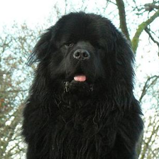
    Every image uses the same trainable table. During training, automatic differentiation follows the classification loss back through the Transformer and the addition eᵢ=cᵢ+pᵢ. For one image, the direct addition gives ∂L/∂pᵢ=∂L/∂eᵢ. When a table is broadcast across a minibatch, its gradient combines contributions from those images according to the loss reduction. The optimizer updates its coordinates together with the patch projection, attention and classifier parameters. Grid slot identity is already known from patch extraction; no extra position-label prediction loss is needed. All coordinates are updated by tensor operations, rather than 196 separately trained models. The SGD numbers are a hand-chosen arithmetic example, not a measured update to the pretrained checkpoint; practical training may use AdamW. Inference performs the additions with the trained table but makes no optimizer updates. Fixed sinusoidal encodings are another design: a deterministic sin/cos function of position and coordinate supplies the vector, so there are no trainable entries for that encoding. The original Transformer studied both choices; the original ViT and this checkpoint use a learned table. The choice is part of the architecture, not something implied by the word position. ViT paper, §3.1 · timm implementation · Original Transformer position encodings.
    Why add CLS? Give the classifier one image summaryA SHORT DETOUR · WHY ADD CLS?One image label from 196 patch rowsWhich representation should the classifier read?The whole dog photo196 patch rowsP1 featuresP2 featuresP196 features⋮ClassifierOne image labelCLS · learned start+Transformerblocksall 197 rowsCLS reads patch featuresFinal CLSimage summaryAveraging final patch rows is another readout option.
    The same dog photograph whose 196 patches must support one image prediction

    Problem: we have 196 patch feature rows, but want one label for the whole photo. Which representation should the classifier read?

    1. Add CLS: reserve an extra learned row before the Transformer blocks.
    2. Gather image information: all 197 rows pass through the blocks. Attention lets CLS read patch features; the patch rows are updated too.
    3. Read final CLS: its updated, image-dependent features go to the classifier, which scores image labels.

    CLS starts as shared model parameters. The next slides show where those numbers come from.

    CLS is one design choice. Averaging the final patch rows is another readout option.

    Patch embeddings give us many rows, while the target is one label for the photograph. We need a way to combine patch information into the representation that the classifier will read.

    The task gives a label for the whole image, while patch embedding has supplied 196 separate feature rows. We need a rule for turning those rows into an image-level prediction. This checkpoint chooses a designated summary row called CLS, short for classification token. Add it before the Transformer blocks so that it can participate in self-attention alongside the patch rows. Its initial learned vector is shared across images; it does not yet contain information about this particular dog. Through attention it receives weighted mixtures of source value vectors, and the blocks transform its representation. The final CLS therefore depends on this image. After the blocks and final normalization, the classifier reads that row to produce class scores. The class-label training loss teaches the model which information makes this readout useful. All patch rows are updated too; this overview follows only CLS at the output. There is no extra image crop, supplied answer label, or separately supervised patch label. CLS is a learned readout mechanism, not a mathematical requirement for image classification. A model can instead average its final patch rows and train a classifier on that vector; the later comparison explains this alternative with the same dog. Position and CLS have separate jobs: position supplies location, while CLS is the row selected for the image-level readout. The next slide compares the origins of patch rows and CLS; we then explain the stored parameters and how training changes them. Original ViT, §3.1.
    Add a summary row beside the dog’s patch rowsThe photograph still has exactly 196 patches.The same dog photoP63768 pixel valuesLinear(768, 192)Patch content c₆₃192 featuresCreate a parameter192 trainable numbersCLS row192 features196 image rows + 1 summary row = 197 rows

    The same dog photograph still gives 196 real patches.

    P63: 16 × 16 × 3 pixels → 768 values → Linear(768,192) → 192 content features.

    CLS: a separately stored parameter → 192 coordinates. It has no pixels and no patch projection.

    196 patch rows + 1 CLS row = 197 rows.

    A patch row comes from pixels. CLS comes from a separate set of model parameters. No extra crop is cut from the photograph. Its 192 coordinates match the width of every patch row.

    The figure compares the origins of the content rows, before position is added. P63 is a real 16×16 RGB crop, projected from 768 values to 192 features. CLS is a separately stored vector of 192 trainable parameters. It bypasses the patch-pixel projection. The model appends no region to the photograph: it prepends a row to the sequence of representations. As the preceding slide showed for patch rows, position is then added; CLS also has its own position vector.
    What makes CLS an image summary?CLS and patch rows can read one another’s current features.Same photoInputShared CLS start196 patch rowsAfter block 1Updated CLSUpdated patch rowsBlock 1After block 2Updated CLSUpdated patch rowsBlock 2197 × 192 at each stage. All updates use that block’s input rows.Continue through block 12. The classifier then reads final CLS.The class loss trains this row to carry useful image information.

    Same dog image → 196 patch rows. Add the shared starting CLS.

    1. Block 1: CLS can read CLS and all patches. Every patch can also read CLS and all patches. All attention outputs use the same incoming rows.
    2. Block 2: its attention reads both the updated CLS and the updated patch rows produced by block 1. The new outputs become the next block’s inputs.
    3. Continue through block 12: every block has its own learned parameters. All 197 rows remain 192 features wide.

    Why a summary? The classifier reads final CLS. The class loss trains the network to make its features useful for predicting the image’s class.

    We do not supply a target summary vector or assign a meaning to each coordinate. The diagram is conceptual; the next slide shows saved values.

    CLS can read all patch rows; each patch can read CLS and every patch. All updates use the rows entering that block. Block 2 reads the updated CLS and patches produced by block 1.

    Follow the same dog through the stack. At the input, CLS is the shared learned start plus its position vector. In block 1, attention brings image-dependent value messages into CLS. The block also updates the patch rows. The purple diagonal makes the reverse information path explicit: patch queries can read the incoming CLS key and value. Within one attention operation, every row’s Q, K and V is computed from the same normalized input sequence. All attention outputs are computed together; a query does not read another row’s newly computed output from that same operation. Block 2 receives all of block 1’s updated rows: its CLS and patch queries, keys and values are computed again from those representations. This continues through 12 successive blocks, each with its own learned parameters. The arrows summarize complete blocks, including attention, residual additions and the per-row MLP; their detailed computation comes later. Both diagonals show possible information flow, not equal attention weights or a guarantee of a large contribution. The horizontal arrows include the within-group dependencies: CLS can read itself, and each patch can read every patch, including itself. There is no causal mask here. All 197 incoming rows are available to every query. All 197 rows retain 192 coordinates. The marks stand for changing features; they are not measured activations or attention weights. The class head reads final CLS after final normalization. During training, the class loss sends gradients through this readout and the blocks, adjusting their weights and the shared starting CLS. There is no target summary vector or instruction assigning “fur”, “eyes” or “breed” to a coordinate or layer. A summary here means a learned representation useful for the classification objective, not a sentence describing the photograph or a copy of every pixel. The objective encourages useful features; it does not guarantee that every block increases confidence. During this saved forward pass, model parameters remain fixed and only the image-dependent activations change. ViT: class token, encoder and classification head.
    The same CLS start reads two different photographsShared learned CLS s = [−0.356, −0.038, −0.072, …]Add the same position vector before either image enters attention.Starting CLS input e₀After attention + residualDog[−0.704, −0.067, −0.146, …]Attentionsame parameters[0.463, −0.118, 0.216, …]196 dog patch rowsCat[−0.704, −0.067, −0.146, …]Attentionsame parameters[0.441, −0.147, 0.254, …]196 cat patch rowsFirst 3 of 192 coordinates shown. Both CLS rows remain 192 numbers wide.

    Shared learned CLS parameter: [−0.356, −0.038, −0.072, …]. Add its shared position vector.

    Dog

    CLS rowFirst three coordinates
    Input[−0.704, −0.067, −0.146, …]
    After first attention + residual[0.463, −0.118, 0.216, …]

    Cat

    CLS rowFirst three coordinates
    Input[−0.704, −0.067, −0.146, …]
    After first attention + residual[0.441, −0.147, 0.254, …]

    Same 192-coordinate input and same model parameters. Different patch rows produce different updates.

    First three coordinates shown. This is the first attention update, before its MLP.

    Both images use the same starting CLS and the same model parameters. Their patch rows differ, so attention produces different updates. These are measured CLS values after the first attention update and residual addition.

    Each displayed CLS input is the same stored parameter plus the same CLS position vector. The 196 patch rows differ with the photograph. The trace checks equality of all 192 CLS input coordinates and the first-block CLS queries for all three heads. Attention compares these queries with image-dependent source keys and mixes image-dependent source values. The displayed output is E + Attention(LayerNorm(E)), at the CLS row, before the first block’s MLP. LayerNorm is included in the measured computation; its details remain in the later complete-block section. All model parameters are held fixed. Values are rounded to three decimals; dots omit 189 coordinates. All 192 coordinates for both photographs · Reproduce this comparison.

    Model route · highlighted operation

    ImagePatchesProjectionPrepare rowsAttentionMLPRead summaryClass scoresinside one block
    Add the summary row: 196 + 1 = 197The full sequence entering block 1CLSlearned token+p₀=e₀1 × 192P1c₁+p₁=e₁1 × 192P63c₆₃+p₆₃=e₆₃1 × 192P196c₁₉₆+p₁₉₆=e₁₉₆1 × 192Stack: [e₀; e₁; …; e₁₉₆] → E has shape 197 × 192
    RowContent + positionShape
    CLSlearned token + p₀1 × 192
    P1c₁ + p₁1 × 192
    ………
    P196c₁₉₆ + p₁₉₆1 × 192

    Stack all rows: E has shape 197 × 192.

    Each patch keeps its content-plus-position row. CLS gets its own learned position too. Stack the summary and patch rows into E: 197 rows, each with 192 features. Batch size one is omitted here.

    The full input is [CLS; C]+P, with 197×192 entries. We already calculated the 196 patch rows C+P_patch. Prepending CLS+p₀ gives exactly the same sequence. The trace verifies this equality against the checkpoint. Its initial CLS row begins [−0.704, −0.067, …]. The ellipsis indicates omitted patch rows; all 196 are present. Measured full-model trace · Reproduce every operation.
    Start with one Transformer blockOur dog photographPrepared rows197 × 192Transformer block 1Attentionshare contextMLPrefine featuresUpdated rows197 × 192Each row keeps 192 features. Its numbers are updated.First, let’s follow this one block.
    The dog photograph whose feature rows enter block 1

    Prepared rows: 196 patches + one CLS → 197 × 192.

    Block 1: attention shares information across rows → MLP transforms each row.

    Output: 197 × 192, with updated feature values. First follow this one block.

    Our 196 patch rows and one CLS row enter block 1. Attention shares information across rows; the MLP transforms each row. The output still has 197 rows and 192 features per row.

    The input E has shape 197×192, with positions already added and CLS already present. This introductory diagram groups each branch’s normalization and residual addition with its named operation; the upcoming attention and MLP slides open those branches. We next inspect Q/K/V for patch 63, then the CLS query and its message, all within block 1. After completing that block, we will pass its output to block 2 and introduce the full stack. Measured full-model trace · Reproduce every operation.
    Self-attention: Q, K and V share the same inputTRANSLATION · cross-attentionTarget-prefix statesQEncoded source statesK, VTwo language streams meet at attention.ViT · self-attentionCurrent CLS + patch statesone image sequenceProject the same rows into Q, K and Vthen mix their informationViT has one stream. Translation had two streams.

    Self-attention uses one input sequence. Cross-attention takes queries from one stream and keys and values from another.

    No. CLS is one row inside the image sequence. In this pre-LN model, all three projections read the same normalized current rows.

    Self-attention uses one input sequence. Cross-attention takes queries from one stream and keys and values from another.

    Photo walkthrough · Step 12 of 12

    ImagePatchesProjectionPrepare rowsAttentionMLPRead summaryClass scoresinside one block
    12 · Make queries, keys and values from these rowsP63: pixels → patch projection → c₆₃ → add p₆₃ → e₆₃All 197 rows are ready. Follow patch 63 into the first block.e₆₃1 × 192LayerNormstill 1 × 192× W_Q + b_Qq₆₃1 × 64× W_K + b_Kk₆₃1 × 64× W_V + b_Vv₆₃1 × 64Each W: 192 × 64; each bias: 64LOCAL ROLESQ / receiverK / sourceV / message
    P6316 × 16 × 3

    Pixels → patch projection → c₆₃ → add p₆₃ → e₆₃

    e₆₃ (1 × 192) → LayerNorm → z₆₃ (1 × 192).

    Head one · separate learned mapsOutput shape
    q₆₃ = z₆₃W_Q + b_Q1 × 64
    k₆₃ = z₆₃W_K + b_K1 × 64
    v₆₃ = z₆₃W_V + b_V1 × 64

    Each W: 192 × 64. Each bias: 64 entries. This model uses three heads.

    LayerNorm rescales a row’s features and keeps its width. We name it here and study its details later. Three learned maps then make Q, K and V; the diagram shows one of three heads.

    In this pretrained pre-LN Transformer, z₆₃=LayerNorm(e₆₃). For head one, q₆₃=z₆₃W_Q+b_Q, k₆₃=z₆₃W_K+b_K and v₆₃=z₆₃W_V+b_V. Each W has row-vector shape (192,64), each bias has 64 entries, and each output is a (1,64) row. The branch boxes show multiplication by the appropriate weight matrix and addition of the corresponding bias. The model’s embedding width is 192 and it uses three heads, so each head has 64 features. Other model choices may use different widths. The checkpoint packs Q/K/V parameters into one layer; our script verifies the head-one slices against the packed result. Every patch follows the same path. The query for this patch is compared with source keys; attention weights then mix source values to update this patch’s representation. That exchange is worked out later in the lecture. Neither patch embeddings nor Q/K/V coordinates are class probabilities. Measured vectors and shapes · Reproduce this trace.

    Model route · highlighted operation

    ImagePatchesProjectionPrepare rowsAttentionMLPRead summaryClass scoresinside one block
    The same input matrix feeds three learned projectionsFollow one head in block 1 · 192 features / 3 heads = 64 per headX = LayerNorm(E)················CLSP1…P19612…192197 × 192·········× W_Q (192 × 64)+ b_Q64 values················CLSP1…P196Q197 × 64·········× W_K (192 × 64)+ b_K64 values················CLSP1…P196K197 × 64·········× W_V (192 × 64)+ b_V64 values················CLSP1…P196V197 × 64LOCAL ROLESQ / receiverK / sourceV / message
    The same dog photograph

    X = LayerNorm(E), shape 197 × 192. Rows: CLS, P1, …, P196.

    Projection from the same XResult
    X W_Q + b_QQ: 197 × 64
    X W_K + b_KK: 197 × 64
    X W_V + b_VV: 197 × 64

    Each W: 192 × 64; each bias: 64. One head, three different learned projections. Row identities stay the same.

    One normalized matrix X feeds three different learned projections. Q, K and V each contain 197 rows of 64 features, in the same token order. This is one head; dots stand for omitted values.

    E is the 197×192 input from the previous slide; LayerNorm changes its values while preserving shape. Call the normalized matrix X. In row-vector notation Q=XW_Q+b_Q, K=XW_K+b_K, V=XW_V+b_V. Each W is 192×64, each bias has 64 coordinates and is broadcast to all 197 rows. These are three affine layers, equivalent to separate nn.Linear(192,64) operations for this head, without an added activation. PyTorch stores each corresponding weight as (64,192); the drawing uses the transposed matrix in XW notation. The checkpoint computes all three heads and Q/K/V jointly with a fused linear layer, then splits the result. Its three heads have distinct parameters. The matrix grids are schematic; dots omit numerical entries, and their equal dimensions do not imply equal values. CLS is first throughout, followed by P1 through P196. ViT paper, Appendix A · This checkpoint’s verified attention computation.

    Model route · highlighted operation

    ImagePatchesProjectionPrepare rowsAttentionMLPRead summaryClass scoresinside one block
    One query–key comparison fills one matrix cellRows: receiving queries. Columns: source keys. CLS is first on both axes.Q · 197 × 64························CLSP1…P63…P19612…64×Kᵀ · 64 × 197························12…64CLSP1…P63…P196Turn K’s rows into columns÷ 8S · 197 × 197Columns = keys →Rows = queries···s································CLSP1…P63…P196CLSP1…P63…P196Highlighted cell: s(CLS, P63) = q(CLS) · k(P63) / 8CLS row: what CLS reads. CLS column: how each query scores CLS.LOCAL ROLESQ / receiverK / sourceV / message

    Q (197 × 64) × Kᵀ (64 × 197) / 8 → S (197 × 197).

    Rows are receiving queries; columns are source keys. Both axes follow CLS, P1, …, P196.

    Which part of S?What stays fixed?What changes?
    CLS row: S[CLS,:]CLS query (receiver)Source key across columns
    CLS column: S[:,CLS]CLS key (source)Receiving query down rows

    For the message that updates CLS, use the CLS row.

    S[CLS,P63] = dot(q_CLS, k_P63) / 8. Sum 64 coordinate products.

    197 × 197 = 38,809 matching scores per head. They can be negative and are not probabilities.

    Fix the receiving query to CLS and move across the columns. These scores determine CLS’s source weights after softmax. Moving down the CLS column changes the query while keeping the CLS key fixed.

    The token order is CLS, P1, …, P196, so 196+1=197. Q has one 64-coordinate query per receiver; Kᵀ has one 64-coordinate key per source column. Contracting the shared 64 dimension produces 197×197 entries, not a sum of the row counts. The highlighted entry uses all 64 coordinate products, scaled by 1/√64. For this dog, P63 is the crop in row 5, column 7 identified earlier. The entry is a learned query–key matching score, not a dog probability or a direct comparison of raw pixels. Q and K use different learned projections, so S(i,j) need not equal S(j,i). The CLS row S[CLS,:] compares one receiving query with every source key; its row-wise softmax supplies the weights for the CLS message. The CLS column S[:,CLS] compares every query with one source key, the CLS key. Its entries belong to different receivers and are normalized within their respective rows. Dots and ellipses denote omitted entries. ViT paper, Appendix A · This checkpoint’s verified attention computation.

    Model route · highlighted operation

    ImagePatchesProjectionPrepare rowsAttentionMLPRead summaryClass scoresinside one block
    Follow the CLS row from scores to weightsS · 197 × 197 scoresColumns = source keys →Rows = queries····································CLSP1…P63…P196CLSP1…P63…P196CLS row, enlargedCLS query stays fixed; compare every source key.zooms₀CLSs₁P1s₂P2……s₆₃P63……s₁₉₆P196softmaxacross all 197 scoresa₀a₁a₂…a₆₃…a₁₉₆a₀ + a₁ + … + a₁₉₆ = 11 CLS score + 196 patch scoresPatch queries update patches → the next block’s CLS reads those updated patches.LOCAL ROLESQ / receiverK / sourceV / message

    Highlight row CLS in S (197 × 197), then enlarge that row.

    Source keyScore for the CLS queryAfter softmax
    CLS itselfs₀a₀
    P1s₁a₁
    P2s₂a₂
    ………
    P63s₆₃a₆₃
    ………
    P196s₁₉₆a₁₉₆

    1 CLS self-score + 196 patch scores = 197 scores. For this fixed CLS query, s_j = dot(q_CLS,k_j) / 8.

    Softmax across all 197 scores gives 197 weights: a₀ + a₁ + … + a₁₉₆ = 1. Each a_j weights the corresponding source value row.

    Why compute the other rows? Each patch gets its own update. The next block’s CLS reads keys and values made from those updated patches.

    Final-block exception: if the classifier uses only final CLS, a specialized implementation could compute only that output. It still needs all 197 incoming keys and values. The standard implementation here computes every row.

    No causal mask: the whole image is available before predicting its class. The ellipses only shorten the drawing; no source is excluded from softmax.

    Earlier blocks update patches so later CLS queries can read their new features. In the final block, a CLS-only readout could compute just the CLS output, using all 197 incoming keys and values.

    The purple outline selects the first row of S, not its first column. The two connecting lines enlarge that same row without changing its contents or order. Here the receiving query is fixed to CLS, so s_j is shorthand for S[CLS,j] = dot(q_CLS,k_j)/8. Source 0 is CLS itself; sources 1 through 196 are the image patches P1 through P196. Ellipses omit scores from the drawing, but all 197 enter the softmax denominator: a_j = exp(s_j) / Σ_{k=0}^{196} exp(s_k). The resulting a_j is shorthand for A[CLS,j], the weight on source j’s 64-feature value row. To calculate this single message in isolation, q_CLS Kᵀ / 8 gives a 1×197 score row; its row-wise softmax multiplied by V gives a 1×64 message. Other query scores are not inputs to this row’s softmax. However, in blocks 1–11 of this model, the other query rows compute the patch updates needed by later blocks. After attention, residual additions and the per-row MLP, these updated patches supply the next block’s keys and values. Keeping only CLS at every block would change the model’s computation. A final-block optimization follows from the same equations: when the only readout is final CLS, one can compute only the CLS query and output in block 12, while still computing keys and values for all 197 incoming rows. The final attention projection, residual update, MLP and normalization can then operate on CLS alone. For the deterministic forward pass here, this preserves the class prediction up to numerical rounding. It does not apply unchanged to patch-level outputs or a readout that pools patch rows. The standard checkpoint implementation used in this lecture computes all rows, including in the final block; actual speed gains from a specialized path depend on the implementation and hardware. These are symbolic entries, not measured outputs. Every source is permitted because the full image is observed before its class label is predicted. The next slide applies the same operation to each of the remaining query rows; later we use the weights to mix V. ViT paper, Appendix A · This checkpoint’s verified attention computation.

    Model route · highlighted operation

    ImagePatchesProjectionPrepare rowsAttentionMLPRead summaryClass scoresinside one block
    Turn each query’s 197 scores into 197 source weightsS: matching scoresA: attention weights···s································CLSP1…P63…P196CLSP1…P63…P196softmaxacross each row···a································CLSP1…P63…P196CLSP1…P63…P196Highlighted CLS row: sum = 1a(CLS, P63): how much weight CLS gives to P63’s value row.LOCAL ROLESQ / receiverK / sourceV / message

    S (197 × 197) → softmax across each row → A (197 × 197).

    The CLS row contains weights for CLS, P1, …, P196. All 197 weights sum to 1.

    A[CLS,P63] = exp(S[CLS,P63]) / sum(exp(S[CLS,k])) over all 197 source rows k.

    It is the coefficient on P63’s value row in the message to CLS. The sources are image rows, not animal classes.

    Apply softmax across each score row. The CLS row becomes weights over CLS and all 196 patches, summing to one. Each other query gets its own weight row. These weights tell us how to mix the value rows.

    A has the same 197×197 shape and token order as S. For receiver i and source j, A[i,j] = exp(S[i,j]) / Σ_k exp(S[i,k]), where k runs over all 197 source rows. A is nonnegative, and each receiver row sums to one in the deterministic forward pass shown. Training-time attention dropout, when used, is a subsequent operation and is not drawn here. The highlighted CLS/P63 weight determines the coefficient on v(P63) in the CLS message. Row-wise softmax does not generally make A symmetric or make its columns sum to one. The later classifier softmax is a different operation over 1,000 image labels. Grid entries are schematic. ViT paper, Appendix A · This checkpoint’s verified attention computation.

    Model route · highlighted operation

    ImagePatchesProjectionPrepare rowsAttentionMLPRead summaryClass scoresinside one block
    Every image row can read every image rowText: predict the next tokenViT: classify the whole image•××××ו•×××ו••××ו•••×ו••••ו•••••t₁t₂t₃t₄t₅t₆t₁t₂t₃t₄t₅t₆••••••••••••••••••••••••••••••••••••CLSP1…P63…P196CLSP1…P63…P196Read the current and earlier positionsRead every row, including itselfFilled cell = permitted connection. × = blocked. This shows access, not weight size.No causal mask here: CLS can read P196, and P196 can read CLS.LOCAL ROLESQ / receiverK / sourceV / message

    Text generation: receiving position t_i may read source positions t_j only when j ≤ i.

    This image classifier: every receiving row may read CLS and P1 through P196.

    There is no causal mask. The whole photograph is available before predicting its label.

    CLS can read P196; P196 can read CLS. Every row can also read itself. Permitted access does not imply equal weights.

    Next-token prediction hides later text positions. Here the complete photograph is available before classification. Every query can use every key and value, including itself. The ViT attention matrix has no causal triangle removed.

    Rows are receiver positions and columns are sources in both access diagrams. t₁…t₆ illustrate six text positions in a causal decoder, where later source positions are masked before softmax. The image axes abbreviate 197 rows with ellipses; every entry in the full 197×197 matrix is allowed. The top-left image entry allows CLS to read itself, the top-right allows CLS to read P196, and the bottom-left allows P196 to read CLS. Allowed access does not imply equal or large attention weights. The fixed-size, fully populated image input used here also has no padding mask. Other architectures may use other masks, but no causal mask is part of this classifier’s saved forward pass. ViT paper, Appendix A · This checkpoint’s verified attention computation.

    Model route · highlighted operation

    ImagePatchesProjectionPrepare rowsAttentionMLPRead summaryClass scoresinside one block
    A message for CLS works like a message for bankChoose a receiver. Mix source values to make a message for that receiver.Text · receiver: bankriverother allowedtokensMix their valuesusing bank’s weightsMessage for bankImage · receiver: CLSP1P63P196…CLSMix their valuesusing CLS’s weightsMessage for CLSSame weighted-sum operation. Different receiver and sources.LOCAL ROLESQ / receiverK / sourceV / message
    ReceiverSourcesResult
    bankriver and other causally allowed tokensweighted value mixture for bank
    CLSP1–P196 and CLS itselfweighted value mixture for CLS

    Same attention operation: use the receiver’s weights to mix source value vectors.

    In text, bank receives a weighted mixture of allowed token values. Here, CLS receives a weighted mixture of image-token values, including its own. The query chooses the receiver; the values supply the message.

    Recall the text-attention message diagram: bank at position 7 uses its query to assign weights to positions 1–7, including river. Those weights mix value vectors into a message for bank. The dog calculation uses the same operation with CLS as the receiver and all 197 image-token rows as permitted sources. The photo crops identify source rows; we mix their projected value vectors, not their pixels. CLS has no crop but participates as both a possible receiver and a source. This diagram describes the computation, not a claim that any named source necessarily gets a large weight. A message is an intermediate vector. The output projection and residual addition will later use it to update the receiving token’s representation. The token’s identity stays the same. Saved P63 value row · Saved CLS weights and message · Saved source contributions and receiver messages · Verified forward computation.

    Model route · highlighted operation

    ImagePatchesProjectionPrepare rowsAttentionMLPRead summaryClass scoresinside one block
    The dog’s feature rows become value rowsSame dog · block 1 · head 1196 patches + CLSX = LayerNorm(E)························CLSP1…P63…P19612…192197 × 192Linear(192,64)× W_V + b_VV: one value row per source························CLSP1…P63…P19612…64197 × 64P63 → v₆₃ = [−0.174, −1.201, …, −1.308]64 learned features · rounded values from this dogLOCAL ROLESQ / receiverK / sourceV / message
    The same dog photograph

    X = LayerNorm(E): 197 × 192. Apply the same Linear(192,64) to every row.

    V = X W_V + b_V: 197 × 64, ordered CLS, P1, …, P196.

    P63’s value row begins [−0.174, −1.201, …] and has 64 learned features.

    Use the same normalized input X that produced Q and K. The value projection makes 64 features for each of its 197 rows. P63’s crop identifies one source; its value row contains learned features.

    This is head 1 of block 1 in the saved dog forward pass. The image’s patch projection and positions already produced E; we do not flatten or project pixels again here. X=LayerNorm(E), then V=XW_V+b_V with W_V shaped 192×64 and a 64-coordinate bias, shared across source rows. There is no additional activation after this value projection. The diagram abbreviates matrix entries; the P63 preview is read from the saved head1_v array, whose length is 64. These coordinates are learned features rather than RGB channels. The displayed dog grid connects source identity to a crop; CLS comes from the extra learned row explained earlier. Saved P63 value row · Saved CLS weights and message · Saved source contributions and receiver messages · Verified forward computation.

    Model route · highlighted operation

    ImagePatchesProjectionPrepare rowsAttentionMLPRead summaryClass scoresinside one block
    One weight scales all 64 features in its value rowA · 197 × 197 weightsColumns = source keys →Rows = queries····································CLSP1…P63…P196CLSP1…P63…P196×V · 197 × 64 valuesColumns = value features →Rows = sources························CLSP1…P63…P19612…641 · Pick receiver CLS2 · Pick source P63a₆₃A[CLS, P63] · one weight0.0005043 · Pick P63’s value rowV[P63, :] · all 64 features×−0.174−1.201…−1.308v₆₃,₁4 · Scale each featureContribution to CLS · 1 × 64=−0.000088v₆₃,₂−0.000606…−0.000659LOCAL ROLESQ / receiverK / sourceV / message
    1. Pick the CLS query row in A (197 × 197).
    2. Pick column P63: A[CLS,P63] = 0.000504.
    3. Pick the matching source row P63 in V (197 × 64).
    4. Multiply feature 1, then repeat for the other 63 features.
    Feature of P63ValueWeight × value
    1−0.174−0.000088
    2−1.201−0.000606
    64−1.308−0.000659

    a₆₃ × v₆₃ → one weighted row of shape 1 × 64. Every feature gets the same scalar weight. Repeat for all 197 sources.

    Receiver: CLS. Source: P63. P63’s own message uses its own query and attention weights.

    Use Next to select CLS’s row in A, P63’s column, P63’s row in V, then its feature coordinates. One scalar scales all 64 values. This contribution is addressed to CLS.

    A has receiving queries on its rows and source keys on its columns. V has the same source identities on its rows, with 64 value features across columns. First select row CLS of A, then column P63. This intersection supplies one scalar A[CLS,P63]. Match that source column to row P63 of V. Select feature column 1 in V and multiply V[P63,1] by the scalar, then repeat for feature 2 through feature 64. The staged diagram keeps both matrices visible; dots abbreviate entries, and the displayed numerical previews are measured. For this fixed CLS query, a_j means A[CLS,j]. Source 0 is CLS itself. The saved weight a₆₃ is 0.0005041293334215879. Its product with the first value feature is -8.759536294384446e-05, and the second product is -0.0006055301711838934. The displayed products use the full stored precision before rounding. The same scalar multiplies all 64 coordinates; no feature dimension is removed. Values may be negative, so weighted features can be negative even though the softmax weights are nonnegative. This crop does not supply a probability for a class; it supplies a learned value vector. Repeat this multiplication for all 197 sources, including CLS. Sending a contribution does not modify P63’s value row. P63’s own update is computed separately from the weights made by its query. The next slide shows four concrete contributions; the following slide adds all 197 sources. Saved P63 value row · Saved CLS weights and message · Saved source contributions and receiver messages · Verified forward computation.

    Model route · highlighted operation

    ImagePatchesProjectionPrepare rowsAttentionMLPRead summaryClass scoresinside one block
    Each source contributes a weighted value rowKeep the receiver fixed: every weight below comes from the CLS row.SourceCLS weightValue row · 64 featuresContribution to CLSCLSCLS0.860556×0.4180.071…0.3598570.060762…P10.002298×−0.211−0.027…−0.000485−0.000063…P630.000504×−0.174−1.201…−0.000088−0.000606…P1960.000233×−1.6071.181…−0.0003740.000275…Four source examples. Every contribution still has 64 features.LOCAL ROLESQ / receiverK / sourceV / message
    SourceCLS weightFirst two value featuresFirst two weighted features
    CLS0.8605560.418, 0.0710.359857, 0.060762
    P10.002298−0.211, −0.027−0.000485, −0.000063
    P630.000504−0.174, −1.201−0.000088, −0.000606
    P1960.000233−1.607, 1.181−0.000374, 0.000275

    Every product is a 1 × 64 contribution to CLS. These four examples are part of the 197-source sum.

    Repeat the P63 calculation for other sources. Each uses its own CLS weight and value row. These are four measured examples from the same head; every contribution is a 64-feature vector addressed to CLS.

    The sources shown are CLS, P1, P63 and P196. Each product uses A[CLS,j] times V[j]. Only two of the 64 coordinates are displayed; the ellipsis means all other features remain. CLS is source index 0 and has a projected value row even though it has no image pixels. These numbers are measured from block 1, head 1 of the trained dog model. The unusually large CLS self-weight in this particular head is a measured result; it is not a general rule for every head, block or image. Products are computed at full precision before rounding. A source contribution does not itself update the source. Next we add all 197 source contributions, keeping the receiving query fixed. Saved P63 value row · Saved CLS weights and message · Saved source contributions and receiver messages · Verified forward computation.

    Model route · highlighted operation

    ImagePatchesProjectionPrepare rowsAttentionMLPRead summaryClass scoresinside one block
    Add the contributions to make one CLS messageAdd the same feature across sources. Keep all 64 features.Weighted contributions for CLS · each 1 × 64CLS0.3598570.060762…P1+−0.000485−0.000063…P63+−0.000088−0.000606…P196+−0.0003740.000275…Other 193+−0.005982−0.003703…Message for CLS0.3530.057…1 × 64197 source contributions → one message for the receiving CLS query.LOCAL ROLESQ / receiverK / sourceV / message
    Source groupWeighted features 1 and 2
    CLS0.359857, 0.060762
    P1−0.000485, −0.000063
    P63−0.000088, −0.000606
    P196−0.000374, 0.000275
    Other 193−0.005982, −0.003703

    Add down each feature column. The complete message begins [0.353, 0.057, 0.024, …], shape 1 × 64.

    Receiver: CLS. This is one head’s message; the embedding update comes next.

    Add corresponding coordinates from all 197 weighted value rows, including CLS itself. The result has 64 features: one message for CLS in this head. The other 193 sources are grouped to keep the addition readable.

    The calculation is h(CLS) = Σ_j A[CLS,j] V[j]. The first four displayed vectors are the same four contributions from the preceding slide. The last vector is the measured sum of the remaining 193 source contributions; it is not a new token or an average. Adding all five displayed vectors gives the complete 64-coordinate message. The saved trace checks this equality at full precision; displayed values are rounded. The first three output features are [0.353, 0.057, 0.024]. Equivalently, (1 × 197) times (197 × 64) gives (1 × 64). This is the weighted-sum operation used for a receiving text token. It produces a context message for CLS, not a class score or the updated CLS embedding yet. Saved P63 value row · Saved CLS weights and message · Saved source contributions and receiver messages · Verified forward computation.

    Model route · highlighted operation

    ImagePatchesProjectionPrepare rowsAttentionMLPRead summaryClass scoresinside one block
    Where does the CLS message go?Same pattern as text: current token row + context update → updated token row.Head 1 messagefor CLS · 1 × 64Combine 3 head messagesthen project to 192 featuresWe open this box next.CLS context update1 × 192Current CLS row1 × 192+Updated CLS row1 × 192The CLS representation changes. It is still the same receiving token.LOCAL ROLESQ / receiverK / sourceV / message

    One head’s CLS message: 1 × 64.

    Combine all three heads’ CLS messages, then apply the output projection: CLS context update, 1 × 192.

    Current CLS row + CLS context update → updated CLS row (all 1 × 192). This is the same residual pattern used for text tokens.

    The CLS messages become a 192-feature context update after combining heads and projecting. Add this update to the CLS row entering the block. The result is a new representation of the same CLS token, as in text.

    This is a destination preview, not an additional attention computation. The middle box takes three messages for the same CLS receiver, one per head, concatenates them into 192 features and applies the learned output projection with its bias. Only head 1’s message is expanded here; the next section shows the other two parallel paths. The current CLS row is the row entering this block, before LayerNorm and attention. The residual path preserves this row until addition: u_CLS = e_CLS + Δe_CLS. The result is an attention-updated activation, which will enter the MLP branch. The stored initial CLS parameter is not changed during this forward pass. As in the text example, contextualizing a token changes its representation while preserving its identity. This particular receiver is later used for image classification. Saved P63 value row · Saved CLS weights and message · Saved source contributions and receiver messages · Verified forward computation.

    Model route · highlighted operation

    ImagePatchesProjectionPrepare rowsAttentionMLPRead summaryClass scoresinside one block
    Each query gets its own messageKeep the source values. Change the receiving query and its weights.ReceiverIts own 197 weightsSame VIts own message · 1 × 64CLS query0.86060.0023…×197 × 640.3530.057…P63 query0.26440.0001…×197 × 640.050−0.358…CLS’s messages update CLS. P63’s messages update P63. Every row has its own.LOCAL ROLESQ / receiverK / sourceV / message
    ReceiverWeights over shared VOne-head message
    CLSA[CLS, all 197 sources][0.353, 0.057, …] (1 × 64)
    P63A[P63, all 197 sources][0.050, −0.358, …] (1 × 64)

    H = A V contains one 64-feature message for each of the 197 receiving rows.

    CLS messages update CLS. P63 messages update P63. All receivers use the same incoming sequence.

    P63’s query mixes the same source values using P63’s weights, producing P63’s own message. CLS and every other patch do the same. Each receiver’s messages ultimately update its own input row through the residual path.

    The two lanes are measured from the same dog, block 1, head 1. Weight previews show source CLS and source P1, followed by the other 195 sources. Both lanes mix all 197 value rows. The receiver is selected by the query, not by which source has the largest attention weight. The full operation H = A V produces 197 rows of 64 features, one message per receiver. Each input row later combines its own three head messages, projects and adds to its own input row. The output projection parameters are shared across receivers. All updates within a block use the same incoming sequence; the newly updated CLS row does not feed P63’s calculation inside this same attention operation. The next block receives the updated sequence. Saved P63 value row · Saved CLS weights and message · Saved source contributions and receiver messages · Verified forward computation.
    From one completed head to three parallel headsHead 1 is complete.Q and K → source weights → mix V → a message for every row.197 input rows197 messages, each 64 featuresNow use three heads in parallelEach reads the same input rowsFirst combine their messages. Then continue to the MLP.

    Head 1 is complete: Q/K → weights → weighted V → H¹ (197 × 64).

    Now follow three parallel heads from the same 197 × 192 input. Combine their messages, project, add E, then continue to the MLP.

    We have finished one head’s attention calculation. This model has three heads. Each starts from the same input rows and computes its own messages. Next, follow those parallel paths and combine their outputs before the MLP.

    This is a topic break within the same real-image forward pass. One head has produced H¹ of shape 197×64, including a 1×64 message for CLS. The chosen checkpoint has three heads. To continue its actual forward pass, compute the other two messages, concatenate all three, project to 192 features and add E. The MLP follows this attention residual. Heads are parallel; Transformer blocks are sequential. Measured three-head CLS trace · Reproduce the head projections and concatenation.
    What might different heads look for in this photograph?Illustrative possibilities · learned heads are not assigned these jobsNearby texturea different weightedmessageDoes this fur continue nearby?Animal partsa different weightedmessageWhich face clues belong together?Wider contexta different weightedmessageHow does this region fit the scene?
    Possible patternExample question
    Nearby textureDoes this fur continue nearby?
    Animal partsWhich face clues belong together?
    Wider contextHow does this region fit the scene?

    Illustrative hypotheses. The classification loss learns the head parameters.

    Different heads can learn different matching patterns and different messages. Local texture, relationships between parts and wider context are possible intuitions. These are hypotheses, not measured head labels.

    Every head receives the same input rows. Its own Q, K and V projections can extract different matching and message features. Heads need not have neat names: they may overlap, mix several cues, or be redundant. We later inspect measured maps without treating them as proof of a semantic role.

    Model route · highlighted operation

    ImagePatchesProjectionPrepare rowsAttentionMLPRead summaryClass scoresinside one block
    The same rows feed three sets of Q, K and V196 patch rows + one CLS row = 197 rowsEach Q/K/V: 197 × 64X = LayerNorm(E)················CLSP1…P196197 × 192Head 1own Q/K/V projectionsQ¹················CLSP1…P196K¹················V¹················Head 2own Q/K/V projectionsQ²················CLSP1…P196K²················V²················Head 3own Q/K/V projectionsQ³················CLSP1…P196K³················V³················One shared CLS input; each head projects it differently.

    X = LayerNorm(E), 197 × 192: CLS plus P1 through P196.

    HeadIndependent projectionsEach result
    1Q¹, K¹, V¹197 × 64
    2Q², K², V²197 × 64
    3Q³, K³, V³197 × 64

    Each projection uses its own W (192 × 64) and bias (64). All heads read the same CLS row and all patches.

    All three heads read the same normalized matrix X. Each has its own Q, K and V projection weights and biases. Every output matrix has 197 rows and 64 features. The highlighted first row is always CLS.

    For head h, Qʰ=XW_Qʰ+b_Qʰ, Kʰ=XW_Kʰ+b_Kʰ and Vʰ=XW_Vʰ+b_Vʰ. Each matrix W has row-vector shape 192×64, and each bias has 64 coordinates. Every projection reads all 192 input features; the heads do not split the patch list or simply take separate 64-coordinate slices of X. Within each projection, weights are shared across rows. Across heads, the parameters differ. The checkpoint evaluates these projections with one fused Linear(192,576), then reshapes into Q/K/V and three heads. The drawing exposes the equivalent separate operations. The same CLS parameter and its position contribute one row of E, which becomes one row of X and is read by every head. Measured three-head CLS trace · Reproduce the head projections and concatenation.

    Model route · highlighted operation

    ImagePatchesProjectionPrepare rowsAttentionMLPRead summaryClass scoresinside one block
    Each head repeats the complete attention calculationHead 1Q¹················197 × 64(K¹)ᵀ················64 × 197S¹················197 × 197A¹················197 × 197V¹················197 × 64H¹················197 × 64×÷ 8softmax×mix valuesHead 2Q²················197 × 64(K²)ᵀ················64 × 197S²················197 × 197A²················197 × 197V²················197 × 64H²················197 × 64×÷ 8softmax×mix valuesHead 3Q³················197 × 64(K³)ᵀ················64 × 197S³················197 × 197A³················197 × 197V³················197 × 64H³················197 × 64×÷ 8softmax×mix valuesEach head has its own matching scores, attention weights and messages.
    HeadScore and weight matricesMessage matrix
    1Q¹(K¹)ᵀ / 8 → softmax → A¹ (197 × 197)A¹ V¹ → H¹ (197 × 64)
    2Q²(K²)ᵀ / 8 → softmax → A² (197 × 197)A² V² → H² (197 × 64)
    3Q³(K³)ᵀ / 8 → softmax → A³ (197 × 197)A³ V³ → H³ (197 × 64)

    The three paths use different learned projections and run in parallel from the same X.

    Within each head, compare Q with K, scale the scores, apply softmax across each row, then multiply by that head’s V. Each path returns 197 messages of 64 features. The heads operate in parallel.

    For each head h, Sʰ=Qʰ(Kʰ)ᵀ/√64, Aʰ=softmax(Sʰ) over source columns, and Hʰ=AʰVʰ. Every head uses full image attention without a causal mask. Each Hʰ has the same receiver-row order: CLS, P1, …, P196. Equal shapes do not imply equal values. Each drawing is schematic; its highlighted first row is CLS except in the transposed K diagram, where the first column is the CLS key. The next slide compares the three measured CLS message rows for the same dog. Measured three-head CLS trace · Reproduce the head projections and concatenation.

    Model route · highlighted operation

    ImagePatchesProjectionPrepare rowsAttentionMLPRead summaryClass scoresinside one block
    One CLS input produces three different messagesFollow the same dog and the same receiving CLS row.CLS row in X · 1 × 192[0.044, −0.011, 0.154, …]same input to every headHead 1 attention[0.353, 0.057, 0.024, …]CLS message · 1 × 64Head 2 attention[−0.091, −0.112, −0.086, …]CLS message · 1 × 64Head 3 attention[−0.002, −0.566, 0.020, …]CLS message · 1 × 64One CLS input row.Three sets of learned projections.

    Shared normalized CLS row: [0.044, −0.011, 0.154, …] (1 × 192).

    HeadMeasured CLS messageShape
    1[0.353, 0.057, 0.024, …]1 × 64
    2[−0.091, −0.112, −0.086, …]1 × 64
    3[−0.002, −0.566, 0.020, …]1 × 64

    One CLS token. Different head projections and attention computations produce three different messages.

    CLS is the same input row for all heads. Their learned projections produce different queries, keys and values, so their attention computations produce different messages. These measured messages each contain 64 features. There is still one CLS token.

    The displayed vectors are measured activations for the dog in block 1. Ellipses omit coordinates; the shared input has 192 features and each output has 64. A CLS message is not separately stored as a learned token parameter: it is computed anew from the current input. There is one stored CLS parameter vector for the model. After projection and residual addition there will be one updated CLS row, not three separate CLS rows. The trace independently verifies each head’s Q/K/V slices using the same normalized CLS row. Measured three-head CLS trace · Reproduce the head projections and concatenation.

    Model route · highlighted operation

    ImagePatchesProjectionPrepare rowsAttentionMLPRead summaryClass scoresinside one block
    Concatenate the three CLS messagesHead 1 CLS message[0.353, 0.057, …]1 × 64Head 2 CLS message[−0.091, −0.112, …]1 × 64Head 3 CLS message[−0.002, −0.566, …]1 × 64[0.353, 0.057, …]features 1–64[−0.091, −0.112, …]features 65–128[−0.002, −0.566, …]features 129–192One joined row · 1 × 192 (64 + 64 + 64)
    Joined feature rangeSource
    1–64Head 1 message
    65–128Head 2 message
    129–192Head 3 message

    Concatenation appends coordinates: (1 × 64), (1 × 64), (1 × 64) → 1 × 192.

    For all queries: concatenate H¹, H² and H³ → joined messages (197 rows × 192 features). No learned parameters in this step.

    Keep all three messages by placing their coordinates side by side. The joined CLS row has 192 features: 64 from head 1, then 64 from head 2, then 64 from head 3. Concatenation has no learned parameters.

    The operation is torch.cat([h_cls_head1,h_cls_head2,h_cls_head3], dim=-1). No softmax, averaging or learned layer is applied during concatenation itself. The trace verifies all 192 coordinates equal the three complete 64-coordinate segments in head order. For all queries, concatenate H¹, H² and H³ along the feature axis to produce the joined message matrix, denoted J, with shape 197×192. The row count stays 197. CLS remains its first row. Measured three-head CLS trace · Reproduce the head projections and concatenation.

    Model route · highlighted operation

    ImagePatchesProjectionPrepare rowsAttentionMLPRead summaryClass scoresinside one block
    Keep the embedding; add the context from attentionOriginalE197 × 192LayerNormXHead 1H¹ · 197 × 64Head 2H² · 197 × 64Head 3H³ · 197 × 64ConcatenateH¹H²H³Joined messages197 × 192Linear(192,192)× W_O + b_OΔEUpdateSkip path: carry the original E unchanged+UUpdatedU = E + ΔEboth 197 × 192Each H contains one message per row: CLS, P1, …, P196.The same residual pattern as text: original embedding + context update.

    Concatenate heads → joined messages (197 × 192) → Linear(192,192) → Delta (197 × 192).

    The joined matrix has 197 rows: CLS plus 196 patches. Each row has 64 + 64 + 64 = 192 features.

    U = E + Delta, still 197 × 192.

    The skip path carries the original E, before LayerNorm, directly to the addition.

    Next: LayerNorm(U) → MLP → add U. The output projection and MLP are different learned layers.

    Follow two paths from E. The heads produce messages; concatenate and project them to make ΔE. The skip path carries E directly to addition. U = E + ΔE is the contextualized representation passed to the MLP.

    Call the joined message matrix J: J=Concat(H¹,H²,H³). It has 197 rows (CLS plus 196 patches) and 192 features per row (64 from each of three heads). J is a name for this matrix; 197×192 is its shape. The output projection is Delta=JW_O+b_O, with W_O shaped 192×192 and a 192-coordinate bias. This affine layer has no additional activation; it can mix coordinates from every head into each output feature. The residual is U=E+Delta, preserving 197×192. The diagram shows the same residual pattern as the text-attention lecture: retain the original representations and add retrieved context. E contains all 196 patch rows and CLS, including position, for the same dog. At later blocks, E denotes that block’s input representations. The skip path bypasses LayerNorm as well as the head computations. Every row receives its own update, including CLS. Next the MLP branch computes U+MLP(LayerNorm(U)); it is separate from this attention output projection. The original photograph has not been re-encoded and the row count has not changed. Measured three-head CLS trace · Reproduce the head projections and concatenation.

    Model route · highlighted operation

    ImagePatchesProjectionPrepare rowsAttentionMLPRead summaryClass scoresinside one block
    The dog’s CLS keeps its input and gains contextSame dog · block 1 · zoom in on the CLS rowEvery vector below contains 192 numbers.Original CLS embedding[−0.704, −0.067, …]e₀ · 1 × 192After concatenation + projection[1.167, −0.051, …]Δe₀ · attention updateskip path+Contextualized CLS[0.463, −0.118, …]u₀ · 1 × 192First coordinate: −0.704 + 1.167 ≈ 0.463Next: MLP → later blocks → final CLS → class scores.LOCAL ROLESQ / receiverK / sourceV / message

    Original CLS: [−0.704, −0.067, …] (1 × 192).

    Projected attention update: [1.167, −0.051, …] (1 × 192).

    Add coordinate by coordinate: [0.463, −0.118, …] (1 × 192).

    Same dog → MLP → later blocks → final CLS → class scores.

    Add the projected attention update coordinate by coordinate to the original CLS embedding. This produces a contextualized CLS row of the same width. It continues through the MLP and later blocks before the classifier reads the final summary.

    These are measured values from the same dog forward pass, rounded to three decimals. The first two residual additions are −0.704+1.167≈0.463 and −0.067−0.051≈−0.118. All 192 coordinates are added in this way. For a patch row, the same formula updates that patch’s representation using its own head messages; for CLS it updates the image-summary row. The illustration follows block 1. Its output is an intermediate representation, not the final class prediction. The next MLP takes LayerNorm(U), transforms features, and adds its own update to U. Subsequent blocks refine these representations before final CLS classification. Measured three-head CLS trace · Reproduce the head projections and concatenation.

    Model route · highlighted operation

    ImagePatchesProjectionPrepare rowsAttentionMLPRead summaryClass scoresinside one block
    Open block 1: attention, then the MLPInput E197 × 192Transformerblock 1Output E¹197 × 192INSIDE BLOCK 1ENormalize → attention → + Eshare context across rowsUNormalize → MLP → add Utransform each row’s featuresE¹OPEN THIS PART NEXTAll three matrices: 197 × 192. One CLS row: 1 × 192.

    Input E (197 × 192) → block 1 → output E¹ (197 × 192).

    1. Normalize → attention → add E: obtain U.
    2. Normalize U → MLP → add U: obtain E¹.

    Both branches update all rows. Each CLS or patch row stays 192 features wide.

    One block makes two updates. Attention lets rows exchange information; the MLP transforms each resulting row. Each branch adds its update to its input. The block receives and returns 197 rows, each 192 features wide.

    For this pre-LayerNorm model, U=E+Attention(LayerNorm(E)), then E¹=U+MLP(LayerNorm(U)). Attention here includes all heads, concatenation and the output projection. Both additions are coordinate by coordinate. E, U and E¹ all have shape 197×192, while a single selected row has shape 1×192. This is still the same dog forward pass. The next drawings open the MLP and then close the entire block before introducing depth. Saved dog forward pass · Check the block computation.

    Model route · highlighted operation

    ImagePatchesProjectionPrepare rowsAttentionMLPRead summaryClass scoresinside one block
    Open the MLP: 192 inputs, 768 hidden units, 192 outputsFollow the dog’s CLS row after LayerNorm.Normalized row1 × 192n₁n₂n₁₉₂⋮Hidden pre-activation1 × 768−0.0910.248z₇₆₈⋮After GELU1 × 768−0.0420.148a₇₆₈⋮MLP update1 × 192−0.100−0.041m₁₉₂⋮Linear(192,768)GELULinear(768,192)192 → 768 → 768 → 192 features · biases in both linear layers
    OperationShape for CLSFirst values
    LayerNorm(u₀)1 × 192n₁, n₂, …
    Linear(192,768)1 × 768[−0.091, 0.248, …]
    GELU1 × 768[−0.042, 0.148, …]
    Linear(768,192)1 × 192[−0.100, −0.041, …]

    Both linear layers include a learned bias. The same parameters process each row.

    Each linear layer connects every input feature to every output unit. GELU transforms each hidden activation. Only a few neurons are drawn; dots omit the rest. The displayed numbers are measured values for this dog’s CLS row.

    Let n=LayerNorm(u₀). The first affine layer computes z=nW₁+b₁, with W₁ shaped 192×768 and b₁ of width 768. Apply GELU to every coordinate: a=GELU(z), still 1×768. The second layer computes m=aW₂+b₂, with W₂ shaped 768×192 and b₂ of width 192. Its output m has shape 1×192, with no activation after this final linear layer. The first two measured values are drawn in the corresponding nodes; the final symbolic node and ellipsis stand for the remaining units. Lines show learned connections, not their weight values. All 197 rows use this same MLP independently. Hidden width 768 is a model choice; it is unrelated to the 768 RGB values in a 16×16 patch. Saved dog forward pass · Check the block computation.

    Model route · highlighted operation

    ImagePatchesProjectionPrepare rowsAttentionMLPRead summaryClass scoresinside one block
    Add the MLP update to finish block 1Same dog · finish the second residual additionThe MLP produces an update for the current CLS row.After attention: u₀[0.463, −0.118, …]1 × 192[−0.100, −0.041, …]MLP update · 1 × 192keep u₀+Block 1 output: e₀¹[0.363, −0.159, …]1 × 192First coordinate: 0.463 − 0.100 ≈ 0.363Do this for CLS and every patch: E¹ = U + MLP(LayerNorm(U)).

    CLS after attention: [0.463, −0.118, …].

    Add the MLP update: [−0.100, −0.041, …].

    Block 1 CLS output: [0.363, −0.159, …] (1 × 192).

    For all rows: E¹ = U + MLP(LayerNorm(U)), with shape 197 × 192.

    Keep the row produced by attention and add the MLP’s update. The result is this row’s output from block 1. Apply the same operation to all 197 rows. Their feature values change; their identities and width stay the same.

    For the dog’s first CLS coordinate, the stored values verify 0.462772608−0.099954687≈0.362817913. For all rows, E¹=U+MLP(LayerNorm(U)), with U and E¹ shaped 197×192. Each row uses the same MLP weights but receives a different update because its input features differ. The MLP does not mix rows: attention has already supplied cross-patch context. The next block receives the complete E¹ matrix, including all 196 patch rows and CLS. Saved dog forward pass · Check the block computation.

    Model route · highlighted operation

    ImagePatchesProjectionPrepare rowsAttentionMLPRead summaryClass scoresinside one block
    Pass the complete output of block 1 into block 2Same dog · carry every updated row forwardInput ECLS· · ·P1· · ·…· · ·P196· · ·197 × 192E¹CLS· · ·P1· · ·…· · ·P196· · ·197 × 192E²CLS· · ·P1· · ·…· · ·P196· · ·197 × 192Block 1Attention + addMLP + addown learned weightsBlock 2Attention + addMLP + addown learned weightsBlock 1’s output is exactly block 2’s input.All 197 rows continue. Both blocks return 192 features per row.

    E (CLS, P1, …, P196) → block 1 → E¹ → block 2 → E².

    Every matrix is 197 × 192. Each block includes attention + residual, then MLP + residual.

    Block 2 has its own learned parameters and receives all the updated rows.

    The entire output matrix continues to the next block: CLS and all 196 patch rows. Block 2 has its own attention and MLP weights. It applies the same sequence of operations to the feature values produced by block 1.

    E¹ is both block 1’s output and block 2’s input. This model has separate block instances, each with its own LayerNorm parameters, Q/K/V projections, attention output projection and MLP layers. The small attention and MLP boxes each include their normalization and residual addition. The displayed matrices abbreviate their coordinates; the highlighted first row tracks CLS. Patch identities stay in the same row order as their representations acquire context. Saved dog forward pass · Check the block computation.

    Model route · highlighted operation

    ImagePatchesProjectionPrepare rowsAttentionMLPRead summaryClass scoresinside one block
    What changes as the rows move through the blocks?Feature values flow forward; each block uses its own parameter set.Einput featuresBlock 1attention + MLPE¹new featuresBlock 2attention + MLPBlock 1 weightsBlock 2 weightsRecomputed in each block:Q, K, V → attention weights → messages → MLP activations → updated rowsLearned weights stay fixed in this forward pass. Training updates them later.
    QuantityWhat happens
    Features, Q/K/V, weights from softmax, MLP activationsRecomputed from each block’s input
    Learned parametersSeparate set per block; fixed during the forward pass
    Rows and output widthCLS + 196 patches; 192 features per row

    Training changes the learned parameters through backpropagation and an optimizer step.

    Each block recomputes queries, keys, values, attention weights and MLP activations from its input. Its learned parameters stay fixed during this forward pass. The next block uses a different parameter set. Matrix dimensions and row identities stay the same.

    The two boxes denote complete parameter sets, including each block’s two LayerNorms, Q/K/V projections, attention output projection and two MLP layers with biases. They are different stored sets, not the same weights being repeatedly overwritten. In a forward pass, the input matrix changes between blocks; consequently the computed attention patterns and hidden activations can change too. Within a block, its MLP and projections share parameters across all token rows. Across depth, this ViT uses separate parameters for each block. Saved dog forward pass · Check the block computation.

    Model route · highlighted operation

    ImagePatchesProjectionPrepare rowsAttentionMLPRead summaryClass scoresinside one block
    Continue through the stack, then classify the imageOne forward pass through 12 distinct Transformer blocksE197 × 192Block 1attention + MLPown weightsBlock 2attention + MLPown weightsBlock 12attention + MLPown weights…E¹E²E¹¹Every arrow carries all 197 × 192 feature values.After block 12 → final normalization → read CLS → class scoresOne image. Twelve blocks. One prediction at the end.

    E → block 1 → E¹ → block 2 → E² → … → block 12.

    All 12 blocks have their own weights. Every block receives and returns 197 × 192 features.

    After block 12: final normalization → select CLS → class scores → one prediction.

    Pass the updated features through blocks 1 to 12 in order. The architecture repeats, with separate learned parameters in each block. After block 12 and final normalization, read CLS and calculate one set of class scores for this image.

    Each block preserves shape 197×192 and has its own parameter set. E¹, E² and E¹¹ label outputs of blocks 1, 2 and 11; the superscript is a block index, not an exponent. The photograph is patchified and projected once before this stack. The trained initial CLS and position embeddings are added once. Later blocks receive the preceding block’s contextual representations. Twelve is this checkpoint’s chosen depth. The final LayerNorm and class head come after block 12; the next slide opens that readout. Saved dog forward pass · Check the block computation.

    Model route · highlighted operation

    ImagePatchesProjectionPrepare rowsAttentionMLPRead summaryClass scoresinside one block
    Select CLS from the final feature matrixThe same dog has now passed through all 12 blocks.After block 12CLS⋯⋯⋯⋯P1⋯⋯⋯⋯…⋯⋯⋯⋯P196⋯⋯⋯⋯197 × 192FinalLayerNormNormalized rowsCLS⋯⋯⋯⋯P1⋯⋯⋯⋯…⋯⋯⋯⋯P196⋯⋯⋯⋯197 × 192Select CLS[−0.144, −0.340, …]1 × 192One image summary192 featuresRead the highlighted row; the patch rows have already supplied context.
    The same dog after the full forward pass

    Block 12 output (197 × 192) → final LayerNorm (197 × 192) → select CLS (1 × 192).

    Final CLS begins [−0.144, −0.340, …]. These are image-summary features.

    After block 12, all 197 rows are still present. Final LayerNorm keeps the same shape. Select the highlighted CLS row: one image summary with 192 features. Its values now reflect information gathered from this dog’s patches.

    The matrix still contains CLS and P1 through P196. Final LayerNorm operates across the 192 features within each row. The classifier takes h=final[:,0,:], a 1×192 vector for this one image. The matrix drawings abbreviate feature entries, while the selected vector shows the measured first two coordinates. The patch rows have contributed through attention; this model’s final head reads only CLS. Batch size one is omitted from the matrix diagrams. Saved classifier calculation · Reproduce the readout from saved CLS.

    Model route · highlighted operation

    ImagePatchesProjectionPrepare rowsAttentionMLPRead summaryClass scoresinside one block
    Open the classifier: 192 features become 1,000 scoresThis checkpoint predicts 1,000 ImageNet classes.CLS features · 1 × 192Class scores · 1 × 1,000−0.144h₁−0.340h₂6.738h₁₉₂⋮15.476Newfoundland11.401Tibetan mastiff10.521briard⋮997 more class scoresnn.Linear(192,1000)192 weights + 1 biasfor each classOne affine layer produces scores. Softmax follows.

    Final CLS: 1 × 192 → nn.Linear(192,1000) → class scores: 1 × 1000.

    Weight matrix: 192 × 1000 in row-vector math; 1000 × 192 in PyTorch. Bias: 1000.

    ClassMeasured score
    Newfoundland15.476
    Tibetan mastiff11.401
    briard10.521

    Every output reads all 192 features. No hidden layer or GELU in this head.

    Every class has one output neuron connected to all 192 CLS features. Each neuron uses its own learned weights and bias to produce a score. Only three of the 1,000 class neurons are drawn. Their scores are measured.

    The operation is z=hW_class+b_class: (1×192)(192×1000)+(1000) gives 1×1000. PyTorch nn.Linear(192,1000) stores its weight tensor transposed, as 1000×192. The head has 192,000 weights plus 1,000 biases. The drawn connections are representative; the omitted 189 inputs and 997 outputs are also fully connected. Input values and class scores come from the same saved dog representation. The output width is the label count used when training this checkpoint. A cat-versus-dog classifier could use Linear(192,2), with weights trained for those two labels. These scores are logits, not probabilities. Saved classifier calculation · Reproduce the readout from saved CLS.

    Model route · highlighted operation

    ImagePatchesProjectionPrepare rowsAttentionMLPRead summaryClass scoresinside one block
    One class score is a weighted sum plus a biasZoom into one output neuron: Newfoundland−0.144h₁−0.340h₂× 0.00682× 0.01947Other 190 weighted featuressum = 15.4822Bias: 0.0017Σ15.4763one class score−0.0010 −0.0066 + 15.4822 + 0.0017 ≈ 15.4763

    Newfoundland: sum all 192 feature × weight products, then add its bias.

    −0.0010 −0.0066 + 15.4822 + 0.0017 ≈ 15.4763

    The same CLS features feed every class, with separate learned weights and biases.

    Multiply each CLS feature by this class’s learned weight. Sum all 192 products and add its bias. For this dog, the Newfoundland neuron produces 15.4763. Every other class performs the same calculation with its own weights and bias.

    For class c, z_c=Σᵢ hᵢWᵢc+b_c, summing all 192 coordinates. This zoom displays the first two feature values and corresponding learned weights, groups the remaining 190 products, and includes the bias. The bottom arithmetic uses products computed before rounding; the displayed inputs and weights are rounded separately. All 192 stored weights for each displayed class are linked in the trace. The readout check reproduces each dot product and matches the dog’s earlier full-model logits. The classifier weights stay fixed during inference; different photographs supply different CLS feature values. Saved classifier calculation · Reproduce the readout from saved CLS.

    Model route · highlighted operation

    ImagePatchesProjectionPrepare rowsAttentionMLPRead summaryClass scoresinside one block
    Turn all 1,000 scores into class probabilitiesThe alternatives are class labels: normalize over all 1,000.Class scores (logits)Class probabilitiesNewfoundland15.47695.73%Tibetan mastiff11.4011.63%briard10.5210.67%997 more classes⋮1.97% across 997 otherssoftmaxall 1,000 scoresp(Newfoundland) = exp(15.476) / sum of exp(all 1,000 scores)≈ 0.9573 · All 1,000 probabilities sum to 1.
    ClassScoreProbability
    Newfoundland15.47695.73%
    Tibetan mastiff11.4011.63%
    briard10.5210.67%

    Other 997 classes: 1.97% combined. Softmax uses all 1,000 scores.

    p(c) = exp(z_c) / sum_j exp(z_j). Select the largest probability.

    Exponentiate each score and divide by the sum over all 1,000 classes. Newfoundland receives 95.73% probability. The displayed classes are only three alternatives; the remaining 997 also enter the denominator. Choose the class with the largest probability.

    For every class c, p_c=exp(z_c)/Σⱼexp(z_j). The actual computation subtracts the largest logit before exponentiation for numerical stability; this leaves the probabilities unchanged. For the winning class the shifted numerator is 1 and the denominator is 1.044641, giving 0.957266. The trace includes all 1,000 logits, so the complete normalization can be checked. The displayed 997-class probability is an aggregate of the omitted alternatives, not another class. Softmax has no learned parameters. The prediction uses argmax; the highest score and highest probability identify the same class. Saved classifier calculation · Reproduce the readout from saved CLS.
    Two softmaxes, two different questionsThe same normalization, applied to two different questionsATTENTION · one queryWhich source rows help?197 scores → softmax over sources → 197 weightsCLS + P1 + P2 + … + P196CLASSIFIER · one imageWhich image label fits?1,000 logits → softmax over labels → probabilitiesNewfoundland, Persian cat, …

    Attention normalizes across 197 source rows for each query and head. The classifier normalizes across 1,000 labels for each image. Both sum to one along their chosen axis; only the second distribution predicts the image label.

    No. It means that one source contributes strongly to that query’s value mixture. The class head later scores labels using the final CLS features.

    Attention normalizes across 197 source rows for each query and head. The classifier normalizes across 1,000 labels for each image. Both sum to one along their chosen axis; only the second distribution predicts the image label.

    For a batch, attention weights have shape B×3×197×197 and class probabilities have shape B×1000. Softmax uses the last axis in both cases, but the axes mean different things. Cross-entropy in the training code accepts logits and includes log-softmax internally.

    Model route · highlighted operation

    ImagePatchesProjectionPrepare rowsAttentionMLPRead summaryClass scoresinside one block
    The same dog now has its final predictionThe same photographFinal CLS192 image featuresLinear + softmax1,000 probabilitiesChoose the largest probabilityNewfoundland · 95.73%Pixels → patches → contextual features → one image prediction.
    The dog classified as Newfoundland

    Final CLS → Linear(192,1000) → softmax → select the largest probability.

    Newfoundland: 95.73% for this photograph.

    The classifier reads the final CLS, scores 1,000 labels, and selects Newfoundland as the most probable class. Its probability for this photograph is 95.73%. We have completed one forward pass from pixels to an image prediction.

    The photograph is the original Newfoundland example used throughout the lecture. Its patches supplied features that were updated through the 12-block stack alongside CLS. The final normalized CLS feeds the learned classifier, and softmax plus argmax gives the image label shown here. The saved classifier-only calculation matches the earlier full forward pass; no training was performed for this illustration. The next section uses smaller numbers so students can calculate the attention mechanism themselves. Saved classifier calculation · Reproduce the readout from saved CLS.
    Optional recap and extra examples

    Load the learned CLS for our dog example

    Load the learned CLS for our dog exampleReturn to the pretrained model used for this dog.Stored CLS parameter s[−0.356, −0.038, −0.072, …]Its learned position p₀[−0.349, −0.030, −0.074, …]+Starting input row e₀ = s + p₀[−0.704, −0.067, −0.146, …]≈First 3 of 192 coordinates · loaded from the saved model · rounded
    192-coordinate rowFirst three coordinates
    Stored CLS parameter s[−0.356, −0.038, −0.072, …]
    + position p₀[−0.349, −0.030, −0.074, …]
    = input e₀[−0.704, −0.067, −0.146, …]

    Saved trained parameters, reused for every image. Rounded previews; 189 coordinates are omitted.

    The saved model already contains the learned CLS vector and its position vector. Add them to form its starting input row. Load these same parameters for every photograph; no pixel values are needed for this row.

    All three previews come from the existing verified checkpoint trace. Each full vector has 192 coordinates. The displayed values are rounded to three decimals; calculate with unrounded numbers. The CLS parameter and its position vector are separate learned parameter tensors. Their sum is the CLS input activation. These parameters stay fixed during inference. The activation will change as it passes through the blocks and reads this image. Saved model values · How these values were checked.

    The dog’s patches turn CLS into this image’s summary

    The dog’s patches turn CLS into this image’s summaryThis dog’s pixels196 patch input rowspixels → features + positionCLS input e₀same learned start12 blocksall 197 rowsRead final CLS192 featuresStarting CLS inputFinal CLS for this dog[−0.704, −0.067, −0.146, …][−0.144, −0.340, −1.348, …]Class headLinear192 → 1,000Final CLS featuresClass scoresh₁h₁₉₂⋮15.4811.40⋮weights+ one bias per classsoftmaxall 1,000Newfoundland95.73%

    The same dog image → 196 patch input rows. Add the shared CLS input row → 197 rows through 12 blocks.

    CLS activationFirst three of 192 coordinates
    At the input[−0.704, −0.067, −0.146, …]
    After the blocks and final normalization[−0.144, −0.340, −1.348, …]

    Final CLS (192 features) → fully connected Linear(192,1000) → 1,000 class scores → softmax → class probabilities.

    Class neuronMeasured score
    Newfoundland15.48
    Tibetan mastiff11.40

    Each class neuron reads all 192 features with its own learned weights and bias. Softmax uses all 1,000 scores. Newfoundland has the highest probability: 95.73% for this photograph.

    The activation changes with the image. The stored starting CLS parameter remains fixed during inference.

    Here is the learned summary for this dog: 192 features read by the class head. Each class neuron combines all 192 features with its learned weights and bias. Softmax gives Newfoundland the highest probability.

    This is the same saved forward pass used elsewhere in the lecture. Initial e₀ includes the CLS position; final CLS includes all 12 blocks and the checkpoint’s final normalization. Each preview shows three of 192 coordinates. The blocks update patch rows as well as CLS. The class head then maps the final 192-coordinate summary to 1,000 ImageNet scores with one affine layer, nn.Linear(192,1000). Each class neuron has 192 learned weights and one bias. The sketch shows the first and last CLS input neurons and two representative class outputs; the omitted 190 input neurons and 998 output neurons are also fully connected. The displayed scores are 15.48 for Newfoundland and 11.40 for Tibetan mastiff, rounded from the saved trace. There is no hidden layer or GELU in this checkpoint’s class head. Softmax uses all 1,000 scores, including the omitted outputs. The 95.73% value is the saved probability for Newfoundland on this image, not test accuracy. The original learned CLS parameter and classifier weights stay fixed during inference. We are not changing the checkpoint or running new inference or training. The upcoming detailed slides explain how Q/K matching and value mixtures produce the updates. Saved class-head weights, scores and probabilities. Saved model values · How these values were checked.

    Read the two final summaries to classify the photographs

    Read the two final summaries to classify the photographsContinue both images through the same 12 blocks and classifier.Final CLS · 192 features[−0.144, −0.340, −1.348, …]Same class head192 → 1,000Newfoundland95.73%Final CLS · 192 features[−2.999, 5.643, −0.745, …]Same class head192 → 1,000Persian cat96.71%The stored CLS parameter stays fixed. Each image produces its own final summary.

    Dog

    Final CLS: [−0.144, −0.340, −1.348, …]

    Newfoundland · 95.73%

    Cat

    Final CLS: [−2.999, 5.643, −0.745, …]

    Persian cat · 96.71%

    Same starting parameter, same 12 blocks, same class head. Different image-dependent final summaries.

    Every summary has 192 coordinates. The class head produces 1,000 scores.

    After all 12 blocks and final normalization, the two CLS representations differ. The same classifier reads each 192-number summary. It predicts Newfoundland for this dog and Persian cat for this cat.

    The previews are measured final CLS representations after all blocks and final LayerNorm. Each has 192 coordinates, with three shown. The shared Linear(192,1000) class head outputs ImageNet scores, and softmax yields the displayed top-class probabilities. The reproducible trace matches both previously published image predictions and the earlier dog CLS trace. These are probabilities for individual photographs, not dataset accuracy. No optimizer step runs. Different inputs are not guaranteed to have distinct representations in general; this measured pair illustrates how context changes CLS. All 192 coordinates for both photographs · Reproduce this comparison.

    With CLS, read the dog’s final summary row

    With CLS, read the dog’s final summary rowSame dog → patches → projection + positions224 × 224 × 3Input rows · 192 features eachCLS · shared startP1 → e₁P63 → e₆₃P196 → e₁₉₆⋮197 × 19212 blocksattention + MLPRead the final CLS rowDog’s final CLS1 × 192Class headLinear(192, 1000)Newfoundland · 95.73%197 rows are updated; the classifier reads the one reserved for the image summary.
    The dog photograph used throughout the lecture

    196 dog patch rows + one CLS row → 197 × 192.

    12 blocks update every row. Read the final CLS → 1 × 192.

    Linear(192,1000) → class probabilities → Newfoundland, 95.73% for this photograph.

    The dog supplies 196 patch rows. Add the shared CLS row, update all 197 rows through the blocks, then read the final CLS. Its 192 features produce the saved Newfoundland prediction.

    This is the already measured classifier, shown again to locate its readout. Each 16×16 RGB crop is projected to 192 features and receives its position vector. The stored CLS parameter also receives its position vector. All 197 rows pass through 12 blocks. The classifier reads the final normalized CLS representation, then softmax gives the saved 95.73% Newfoundland probability for this photograph. Intermediate normalization is folded into this overview. The patch thumbnails identify rows; the network processes their feature vectors. Saved forward-pass evidence.

    Without CLS, combine the dog’s final patch rows

    Without CLS, combine the dog’s final patch rowsSame dog → patches → projection + positions224 × 224 × 3Input rows · 192 features eachOnly the patch rowsP1 → e₁P63 → e₆₃P196 → e₁₉₆⋮196 × 19212 blocksattention + MLPCombine the final patch rowsMean pooling196 × 192 → 1 × 192Class headLinear(192, 1000)1,000 class scoresTrain this design with image labels, such as Newfoundland for a dog photograph like this.
    The same dog, now used to explain a model without CLS

    196 dog patch rows → 196 × 192 through the Transformer blocks.

    Mean pooling: average final patch features across the 196 rows → 1 × 192.

    Linear(192,1000) → class scores. Train with the breed label Newfoundland for a labelled photo like this.

    This is a proposed model design, with no measured prediction shown.

    Build a second design with 196 patch rows and no CLS. Attention still lets the patches share information. Average their final features to get one 192-number summary. Train the classifier and blocks with this readout.

    This is an architectural alternative, not a measured run of a second model. The known breed label is a supervised training target, not a claimed prediction or an input to the forward pass. Use 196 positional vectors for 196 patch rows; there is no CLS row. The final patch features have already exchanged context through attention. Mean pooling reduces the row axis from 196 to one and preserves all 192 feature coordinates. The classifier has the same input/output dimensions as before, but its parameters and the encoder are trained for the chosen readout. Normalization follows that architecture and is omitted from this overview. No alternate-model accuracy or probability is claimed. ViT paper, Appendix D.3: class token and average pooling.

    Mean pooling: average each feature across the patches

    Mean pooling: average each feature across the patchesSmall calculation · 4 large patches, 2 final features each · chosen numbersP1P2P3P4Same dog, smaller exampleAfter the attention blocksP120P242P324P402Average down each column(2 + 4 + 2 + 0) / 4 = 2(0 + 2 + 4 + 2) / 4 = 2Image summary: [2, 2]4 × 2 → 1 × 2For our full-size design: average 196 rows, keeping all 192 feature coordinates.
    The same dog is split into four large patches for a small arithmetic example

    Separate small example: four large patches and two final features. These numbers are chosen for calculation.

    Patch row after the blocksFinal features
    P1[2, 0]
    P2[4, 2]
    P3[2, 4]
    P4[0, 2]

    Feature 1: (2 + 4 + 2 + 0) / 4 = 2.

    Feature 2: (0 + 2 + 4 + 2) / 4 = 2.

    Image summary: [2, 2]. Shape 4 × 2 → 1 × 2.

    For the full design: 196 × 192 → 1 × 192. Average final features, after attention.

    Each row is a patch representation after it has read context. Average feature 1 across patches, then feature 2. Four rows become one row. In the full model, 196 rows become one 192-feature summary.

    This separate miniature illustration uses four 112×112 crops of the same 224×224 photograph and two feature coordinates per final row. It does not change the real model’s 16×16 patch size or D=192. The four output vectors [2,0], [4,2], [2,4], [0,2] are deliberately chosen arithmetic values, not measured embeddings or outputs from the other worksheet. Their coordinate-wise average is [2,2]. The thumbnails identify which patch each row belongs to; each final row can contain context from all patches. In the full pooling design, for every feature j, summary[j] = (H[1,j] + … + H[196,j]) / 196. In batched code, H.mean(dim=1) maps (B,196,192) to (B,192). Pooling has no trainable parameters; the encoder and classifier learn.

    Why is CLS a common choice if pooling also works?

    Why is CLS a common choice if pooling also works?1 · A familiar conventionBERT: classification tokenOriginal ViT adopts itOur checkpoint uses CLS2 · A dedicated summary, refined through the blocksPatch rows + CLSattentionUpdated CLSlater blocksFinal CLS→ class headAttention learns how to weight sources; the label loss trains the summary.3 · Both readouts deserve a fair comparisonOriginal ViT found similar performance after tuning each readout’s learning rate.ViT paper · §3.1 and Appendix D.3, Figure 9
    1. History: BERT’s classification token → original ViT → our checkpoint.
    2. Role: CLS is a dedicated summary updated through attention; classification loss trains it to support the image label. Patch rows are updated too.
    3. Evidence: the original ViT study found similar performance for CLS and mean pooling after tuning their learning rates. CLS is not a universal accuracy winner.

    Keep the readout used by a pretrained checkpoint. Train or adapt and evaluate a different choice.

    ViT paper, Appendix D.3: class token and average pooling.

    This diagram follows CLS; patch rows receive updates too. Keep the readout a checkpoint was trained to use, or adapt and evaluate the changed model.

    The original ViT adopted the classification-token convention from BERT (§3.1). CLS provides a designated place for the classifier to read an image-level representation. In each block its attention weights can depend on the current query and source keys; later CLS queries already contain image context. The classification objective trains the initial CLS parameter and the shared encoder and classifier weights. The diagram follows the CLS readout only; patch rows also attend to all rows and receive updates. A learned readout is a useful architectural option, not proof of superior accuracy. Appendix D.3 and Figure 9 report comparable class-token and global-average-pooling results once learning rates were tuned. Mean pooling has fixed averaging coefficients over final rows, but those rows contain learned context; it does not make every raw pixel equally important. For an existing checkpoint, retain its readout unless you adapt and evaluate the changed model. We now return to our checkpoint’s 197-row CLS route. ViT paper, Appendix D.3: class token and average pooling.
    Optional reference and extra examples

    Create 192 trainable numbers for CLS

    Create 192 trainable numbers for CLSThe model uses 192 features per row.Give the extra row the same width.s₁1s₂2s₃3……s₁₉₂192Initialize once with small random values; mark them trainable.cls = nn.Parameter(torch.randn(1, 1, 192) * 0.02)

    Choose the same width as each patch row: 192 features.

    Create s = [s₁, s₂, …, s₁₉₂] once, before training.

    cls = nn.Parameter(
        torch.randn(1, 1, 192) * 0.02
    )

    This illustrative code initializes a trainable parameter with small random values. It does not read pixels.

    Shape: one shared batch entry × one token × 192 features. Reuse the same starting parameter across images.

    Before training, initialize one 192-number vector. It is stored in the model, like a learned token embedding in text. The numbers do not come from this photograph. Training will adjust them.

    The code is one illustrative initialization, not a reconstruction of the checkpoint’s original training run. nn.Parameter registers values that can receive gradients and be updated by the optimizer. The tensor shape (1,1,192) means a singleton batch axis, one CLS token and 192 features. Expand the leading singleton axis for a batch; this shares the same parameter across all images. The row width is a model choice, not the number of pixels, patches or classes. Some implementations initialize CLS differently. At inference, load the trained values instead of drawing new random numbers.

    The image label teaches the starting CLS numbers

    The image label teaches the starting CLS numbersTraining idea · imagine this is a labelled training exampleDog photographPatch rows + CLSTransformer blocksClass scorespredictionCompare with labellossKnown labelNewfoundland192 starting CLS parametersadjusted by the optimizerbackward through classifier + blocksThe loss trains CLS along with the other trainable model parameters.

    Illustrative training pair: dog photograph with the label Newfoundland.

    Patch rows + CLS → blocks → class scores → compare with the known label → loss.

    Loss → backward through the model → CLS gradient → optimizer updates its 192 parameters.

    The label is used only in the loss. Repeat across many labelled images; other trainable parameters also learn.

    The label supplies a loss on the prediction. Backpropagation reaches the starting CLS vector through the classifier and blocks. The optimizer adjusts its 192 parameters, along with other trainable weights, across many labelled images.

    This is a teaching illustration of supervised training, not a claim that this specific photo was used to train the saved checkpoint. Use a labelled Newfoundland photograph as an example training pair for the 1,000-class model. The known label enters the loss, not CLS or the forward input. Gradients travel from the loss through the class head and all Transformer blocks to the shared starting parameter. An optimizer then updates that parameter. There is no separate target vector or hand-written dog code for CLS. This diagram highlights one parameter group; other trainable parameters receive gradients too. We are describing the procedure, not running training.
    04

    Optional whole-model walkthrough

    Section 4 · Whole model walkthroughSECTION04Whole model walkthroughWe have opened each part of the classifier.How do forward and backward fit together?

    One example: follow the full model to a label loss, then reverse the path to compute gradients and update the parameters.

    Connect the previous result to this new question. Keep the same image classifier as the reference.

    One example: follow the full model to a label loss, then reverse the path to compute gradients and update the parameters.

    One shape trace from pixels to class scoresONE IMAGE · batch axis omittedPixels3 × 224 × 224Patch projection196 × 192Add CLS + position197 × 19212 encoder blocks197 × 192Final LN → read CLS192Class head1,000 logits

    Blocks preserve the shape. They change what each row represents.

    Prepending CLS changes 196 rows to 197. The head maps the selected 192-feature row to 1,000 logits. Expand the next diagram to see inside every block.

    Blocks preserve the shape. They change what each row represents.

    Inside each block: mix, transform, keep the residualONE PRE-LAYERNORM BLOCK · input and output: 197 × 192ELayerNormSelf-attention3 heads · 64 features each+UULayerNormMLP192 → 768 → 192 · GELU+Carry the input along the skip pathE′Attention mixes rows. The MLP transforms each row. Both add a residual update.

    Repeat this structure 12 times, with different learned weights in each block. All 197 rows are updated in parallel.

    Self-attention mixes value rows. The MLP is applied independently to each row. LayerNorm precedes each branch; residual additions preserve the current representation.

    Repeat this structure 12 times, with different learned weights in each block. All 197 rows are updated in parallel.

    Reusable block diagram (SVG). The full model reference below expands the attention heads, classifier and label loss.
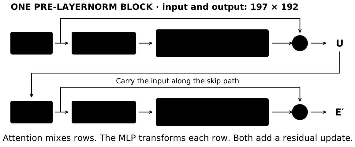
    Backward: compute gradients, then update the modelSame model, reverse direction: loss → parameter gradientsImage x3 × 224 × 224Input embedding197 × 19212 blocks197 × 192Read CLS + head192 → 1,000Label lossL = 0.0437Fixed dataGradients reach the head, all blocks, and the learned input parameters.Compute gradientsθ.grad = ∂L/∂θOptimizer stepθ ← θ − η ∇θ LNext forward passuse updated parametersbackward() computes gradients; step() changes the parameters.

    Label loss → class head and final CLS → blocks 12 through 1 → learned input parameters.

    Gradients reach the head, attention and MLP weights, normalization parameters, patch projection, position table and starting CLS. Input image and label remain fixed.

    backward(): compute θ.grad. step(): update parameters. For SGD, θ ← θ − η∇θL. Then run a new forward pass.

    Reverse the forward dependencies to compute gradients for the trainable parameters. The optimizer uses these gradients to update them. The next forward pass uses the updated model. The image and its label remain fixed.

    The probability is from the saved dog forward pass. Treat this as an illustrative labelled example; we do not claim that this photo was in the checkpoint training set. No training is run. This is the backward pass for the scalar cross-entropy loss in the optional complete-model reference. Start with dlogits=p−one_hot(y). The head receives parameter gradients and passes a gradient to final CLS. Reverse final normalization and the 12 blocks. Residual additions send gradients along both paths, and shared inputs accumulate their contributions. Attention connects the CLS loss to patch keys and values; earlier patch updates can affect later CLS states. Input gradients reach the shared patch projection, the position table and starting CLS. The optimizer is given model parameters, not image pixels. The diagram summarizes these dependencies without opening each block again. The displayed update is ordinary SGD, with learning rate η; other optimizers use the same gradients with their own update rules. In a training loop, zero_grad clears accumulated gradients before backward, and step changes the selected parameters. The parameter update is illustrative, not an executed training result. Saved prediction used in this example.
    Optional reference and extra examples

    The whole Vision Transformer in one figure

    The whole Vision Transformer in one figure1 · RGB image3 × 224 × 22416 × 16 patchesflatten → 196 × 768Shared projection768 → 192 + biasPrepend learned CLS196 + 1 = 197 rows+ learned positionsE⁰: 197 × 1922 · Blocks 1–12 · all 197 rows, each 192 features wide123456789101112E¹²INSIDE BLOCK 1Blocks 2–12 repeat these operations with their own weights.skip: EE197 × 192LN 1197 × 192Head 1: QKVeach 197 × 64QKᵀ / √64197 × 197A = softmaxover source keysAV197 × 64VHead 2: QKVeach 197 × 64QKᵀ / √64197 × 197A = softmaxover source keysAV197 × 64VHead 3: QKVeach 197 × 64QKᵀ / √64197 × 197A = softmaxover source keysAV197 × 64VConcat3 × 64 = 192W_O + b192 → 192+U3 parallel headsNo causal maskU197 × 192LN 2197 × 192MLP: Linear + bias192 → 768GELU197 × 768Linear + bias768 → 192+skip: UE¹197 × 1923 · After block 12: normalize → CLS → class scores → prediction / lossFinal LN197 × 192Select CLS1 × 192Linear head + bias192 → 1,000 logitsSoftmax1,000 probsNewfoundlandtop label · 95.73%Label lossL = 0.0437Cross-entropy(logits, y) · y = Newfoundland
    1. RGB image (3 × 224 × 224) → 196 flattened patches (196 × 768) → shared projection (196 × 192).
    2. Prepend learned CLS and add learned positions: E⁰ is 197 × 192.
    3. Pass all rows through blocks 1–12. Each has separate learned weights.
    4. Inside each block: LN₁ → three parallel attention heads. Each forms Q, K, V (197 × 64), QKᵀ/√64 (197 × 197), row softmax, then AV (197 × 64). Join the heads, project to width 192, and add E to get U.
    5. LN₂(U) → Linear(192,768) → GELU → Linear(768,192) → add U.
    6. After block 12: final LayerNorm → select CLS (1 × 192) → class head (1,000 logits) → softmax → top label.

    The known label y enters only at the loss. Here y = Newfoundland, p(y) = 0.95727, and L = −log p(y) = 0.0437.

    Forward computes activations and loss. Model parameters remain fixed during this calculation.
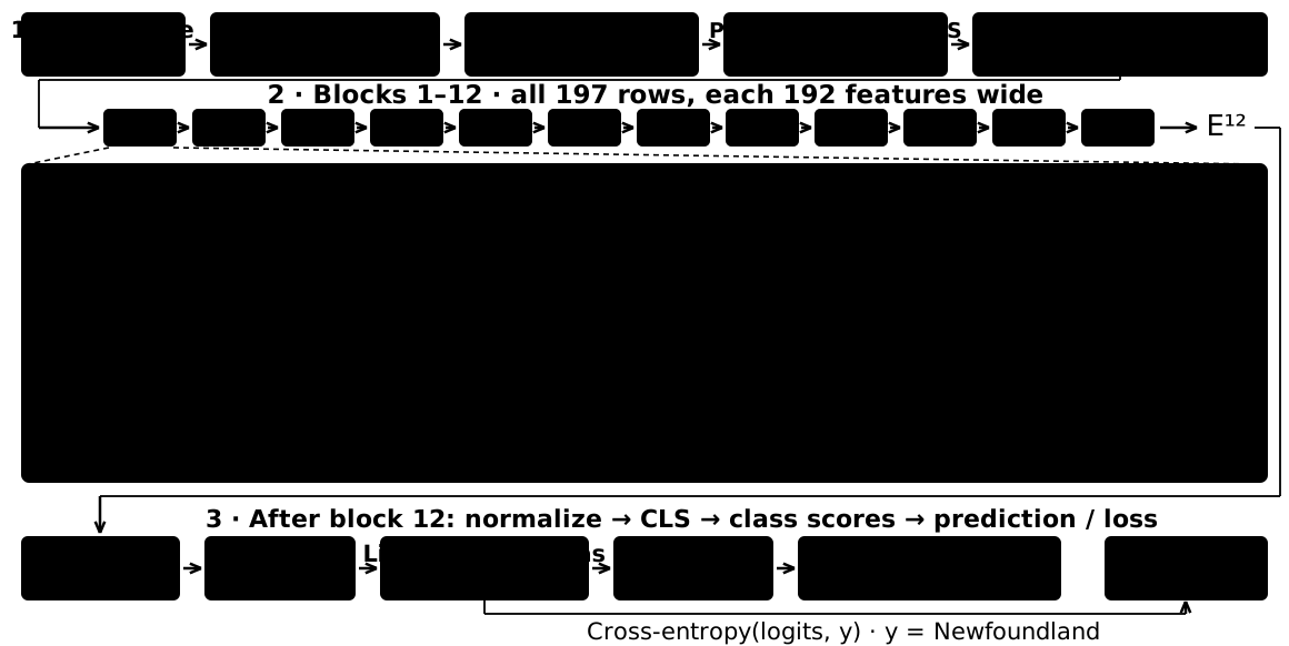
    Open the complete vector diagram.

    Follow the numbered path. The expanded block shows three parallel heads, both residual additions, and the MLP. All 12 blocks keep every row. Final CLS feeds the classifier; the known label enters only at the loss.

    The probability is from the saved dog forward pass. Treat this as an illustrative labelled example; we do not claim that this photo was in the checkpoint training set. No training is run. This complete reference diagram uses the parallel head lanes of the earlier TinyStories map. The single-image batch axis is omitted. Flatten each 3×16×16 patch to 768 numbers; the shared affine projection produces 196 rows of width 192. Prepend the learned 1×192 starting CLS, then add the learned 197×192 position table. All twelve block instances are shown explicitly. The large panel is an expanded view of block 1, not an extra block inserted into the sequence. Each block has its own learned weights and recomputes activations from its input. LN means LayerNorm. With X=LN₁(E), each of the three heads forms its own Q, K and V, each 197×64. Scores QKᵀ/√64 and attention weights A are 197×197; softmax runs across the source-key axis. The dashed V route bypasses scores and softmax. AV returns a 197×64 message matrix per head. Concatenate the three outputs to 197×192, apply the affine output projection, then add E to get U. The second sublayer applies LN₂(U), Linear(192,768), GELU and Linear(768,192), then adds U. Both linear layers have biases. The MLP is shared across rows and does not mix rows. Both residual paths preserve their own sublayer input. Every block returns all 197 rows. After block 12, apply final LayerNorm and select the CLS row. The class head produces 1,000 logits; the displayed probability comes from their softmax. The label is Newfoundland in this example, so L=-log p(Newfoundland). Use the unrounded stored probability to calculate the loss. In PyTorch, cross_entropy takes logits and the label directly. This example illustrates the learning objective; one image’s loss does not establish generalization. Saved prediction used in this example. Open the complete vector diagram.
    05

    Optional CNN comparison

    Section 5 · CNNs, ViTs and inductive biasSECTION05CNNs, ViTs and inductive biasAttention lets patches exchange information.How do they differ, and which should we try?

    Compare context, mixing, wider views and readouts, then connect those choices to inductive bias and practical data and compute constraints.

    Connect the previous result to this new question. Keep the same image classifier as the reference.

    Compare context, mixing, wider views and readouts, then connect those choices to inductive bias and practical data and compute constraints.

    Two ways to build an image representation1 · Gather context: which inputs can interact in one layer?CNN · local filtersViT · global attentionOne local neighbourhoodfeeds one output location.Start with nearby clues.One query can useevery source patch.Near and far are available.2 · Mix information: what determines each contribution?Learned filterReuse the same weightsat every image location.Query + keysCompute weightsfor this query + image.Both learn parameters. ViT recomputes attention weights from the current features.
    PointCNNViT
    1. Gather contextOne output uses a local neighbourhood.One query can use near and distant patches.
    2. Mix informationThe learned filter is reused at every location.Query–key matches determine the source weights for this input.

    First compare the available connections. Then press Next to compare the mixing weights. CNN filters stay fixed during a forward pass. ViT projection parameters also stay fixed, while attention weights are computed from the current query and source features.

    First compare the available connections. Then press Next to compare the mixing weights. CNN filters stay fixed during a forward pass. ViT projection parameters also stay fixed, while attention weights are computed from the current query and source features.

    This compares a conventional CNN with the plain global-attention ViT in this lecture. The neighbourhood and patch arrows are schematic, not measured responses. A convolution computes weighted sums using a learned kernel reused across spatial positions. Its activations still change with the image. In ViT, learned Q/K/V projections stay fixed during inference, but the resulting query/key vectors and attention coefficients are input-dependent. Value vectors supply the features that the coefficients mix. This distinction concerns spatial mixing; both systems also contain nonlinear feature transformations. The next slide follows the wider context and readout. ViT: architecture and spatial assumptions.
    A wider view, then one image label3 · Build a wider view: how do distant clues meet?CNN · local filtersViT · global attentionLocal featuresCombine themWider contextSuccessive layers connect larger regions.Near + farpatchesOne globalattention layerLater blocks refine those relationships.4 · Read out a label: turn many locations into one vector.Spatial averageone feature vectorClass headimage scoresCLSP1…P196Read final CLSone feature vectorClass headimage scoresBoth produce an image-level summary. Pooling is also a valid ViT readout.
    PointCNNViT
    3. Build a wider viewSuccessive local layers combine larger regions.A global attention layer connects distant patches; later blocks refine the features.
    4. Read out one labelOften average the final spatial features, then apply a class head.This model reads final CLS, then applies a class head. Pooling is another option.

    Trace context through the layers, then press Next to inspect the readout. Both models can use the whole image. A classifier needs one image-level vector: CNNs often use spatial pooling; this ViT reads final CLS.

    Trace context through the layers, then press Next to inspect the readout. Both models can use the whole image. A classifier needs one image-level vector: CNNs often use spatial pooling; this ViT reads final CLS.

    The CNN chain is schematic: depth, kernel size, stride and dilation determine its receptive field. Global attention permits a direct dependency between distant patches within a layer, without guaranteeing that a trained head assigns every distant patch a large weight. Both models still need learned features and useful training. A common CNN readout averages each channel across spatial locations; it preserves the feature/channel axis for the classifier. This ViT selects the final normalized CLS row. Its other rows have helped build that summary through attention. Mean pooling is another valid ViT design when the model is trained for that readout. ViT: architecture and spatial assumptions.
    Inductive bias: a useful starting assumptionInductive bias = assumptions built into how the model learns.Example: movethe same stripe.new locationSame localpatternWhat is built in?CNNViT · global attentionSpatial structureLocal filters, reusedacross the imagePatches + position;flexible global mixingThe shifted stripeThe same filter candetect it elsewherePosition can changethe attention patternLearned from dataWhich local filters helpWhich patch relations help
    ComparisonCNNViT
    Spatial structureLocal filters, reused across the imagePatches + position; flexible global mixing
    The shifted stripeThe same filter can detect it elsewherePosition can change the attention pattern
    Learned from dataWhich local filters helpWhich patch relations help

    A CNN builds in local reuse: one learned detector can look for a pattern at many locations. ViT also has structure—patches, shared projections and position signals—but gives attention more freedom to learn spatial relationships.

    A CNN builds in local reuse: one learned detector can look for a pattern at many locations. ViT also has structure—patches, shared projections and position signals—but gives attention more freedom to learn spatial relationships.

    The highlighted neighbourhood is identical before and after the shift, so a shared local filter can reuse its response. Exact convolutional shift equivariance depends on stride and boundaries; it does not guarantee an unchanged final class prediction. ViT shares projection parameters across rows too. Its position signals can affect matching after a shift. The table describes architectural preferences, not hard limits on what either model can learn. ViT: architecture and spatial assumptions.
    Which is a sensible starting point?Practical starting points · validate on your task and hardware.Your situationCNNViT · global attentionFew labels;train from scratchUseful baseline:built-in local reusePay close attentionto the training recipeFew labels;pretrained weightsFine-tune a suitablepretrained CNNFine-tune a suitablepretrained ViTWPhone or tightlatency budgetTry a compact CNN;measure on the deviceTry an efficient ViT;measure on the deviceDistant cluesacross the imageUse enough depthfor broad contextGlobal attention linksdistant patches directlyCompare validation accuracy, speed and memory under the same budget.
    SituationCNN starting pointViT starting point
    Few labels; train from scratchUseful baseline: built-in local reusePay close attention to the training recipe
    Few labels; pretrained weightsFine-tune a suitable pretrained CNNFine-tune a suitable pretrained ViT
    Phone or tight latency budgetTry a compact CNN; measure on the deviceTry an efficient ViT; measure on the device
    Distant clues across the imageUse enough depth for broad contextGlobal attention links distant patches directly

    Treat these as starting points, not a ranking. Pretraining can matter more than the architecture name on a small dataset. Compare suitable models using the same validation set and measure speed and memory on the target hardware.

    Treat these as starting points, not a ranking. Pretraining can matter more than the architecture name on a small dataset. Compare suitable models using the same validation set and measure speed and memory on the target hardware.

    These are practical recommendations inferred from architectural differences and published studies, not results from a new benchmark. The original ViT benefited from large-scale pretraining. DeiT subsequently demonstrated competitive transformers trained on ImageNet without external data, showing why the training recipe matters. Modern CNNs such as ConvNeXt also remain competitive. There is no universal image-count threshold or architecture winner. Model size, resolution, checkpoint suitability, augmentation and implementation affect the comparison. ViT: architecture and spatial assumptions · DeiT: the training recipe matters · ConvNeXt: modern CNNs remain competitive.
    06

    Implementation lab · optional

    Implementation lab · optionalIMPLEMENTATION LAB · OPTIONALBuild the same ViT in PyTorchOne imageB × 3 × 224 × 224Code + tensor shapesLinear and Conv2dThe same predictionB × 1,000Use this lab in class, or work through it after the conceptual lecture.

    All implementation details are retained. Every operation is paired with shapes, diagrams or a numerical equivalence check.

    Exactly the same affine map with the same weights and biases, up to floating-point roundoff.

    All implementation details are retained. Every operation is paired with shapes, diagrams or a numerical equivalence check.

    Keep the same photograph and add the batch axis# rgb: (224, 224, 3), RGB per pixelx = rgb.permute(2, 0, 1) # 3, 224, 224x = x.unsqueeze(0) # 1, 3, 224, 224# Patch order: all R, then G, then BHeight × width × RGBPyTorch: B × C × H × WB × 3 × 224 × 224
    # rgb: (224, 224, 3), RGB per pixel
    x = rgb.permute(2, 0, 1)  # 3, 224, 224
    x = x.unsqueeze(0)       # 1, 3, 224, 224
    # Patch order: all R, then G, then B

    The leading axis B. One photograph uses B=1; a batch of photographs uses the same model parameters for each.

    The prepared photograph is 224×224 with three RGB channels. PyTorch puts channels before height and width, then adds a batch axis. B counts images; it does not count patches.

    The code keeps the lecture architecture: patch size 16, D=192, three 64-wide heads, 12 blocks and 1,000 outputs. It is randomly initialized; the saved dog prediction uses a separate pretrained checkpoint. Here rgb is already a resized/cropped, float, checkpoint-normalized H×W×3 tensor. permute changes axis order, not pixel values. Use the checkpoint’s prescribed normalization for pretrained inference. The diagram shows the saved model-input crop for continuity; this snippet does not run inference.Complete teaching implementation.
    Our target: turn every patch into 192 featuresImplement the same patch projection we used for the dog.224 × 224 × 3196 patchesOne RGB patch3 × 16 × 16= 768 numbersShared projection768 → 192Patch row192 featuresApply the same learned weights and biases at every location.One image → 196 rows, each with 192 features.Two implementations: flatten + Linear or Conv2d

    Each RGB patch supplies 768 numbers. One shared projection turns it into 192 features. Reusing that projection across the 14×14 grid produces 196 rows. We will implement this exact operation in two ways.

    No. Each patch supplies different inputs to the same learned projection. The same parameters also serve the cat and every other image.

    Each RGB patch supplies 768 numbers. One shared projection turns it into 192 features. Reusing that projection across the 14×14 grid produces 196 rows. We will implement this exact operation in two ways.

    This continues the existing 224×224 photo example. We are implementing the patch projection before CLS, position addition and attention. The highlighted location is P63. There is no attention or cross-patch mixing here. Runnable dog/cat equivalence example · Measured outputs and checks. PyTorch Linear · PyTorch Conv2d · PyTorch Unfold.
    See the patch projection as a layer of neuronsOne affine layer: nn.Linear(768, 192, bias=True)768 inputs192 outputsw₁,₁, w₁,₂, …, w₁,₇₆₈x₁x₂x₇₆₈c₁c₂c₁₉₂⋮⋮+ b₁Open just the first output neuronc₁ = w₁,₁x₁ + w₁,₂x₂ + …+ w₁,₇₆₈x₇₆₈ + b₁Every output has its own768 weights + 1 bias.192 × 768 weights + 192 biases = 147,648 parametersPatch projection: no hidden layer or activation. Later MLP: Linear → GELU → Linear.
    QuantityCount
    Inputs per patch3×16×16 = 768
    Output neurons192
    Weights192×768 = 147,456
    Biases192
    Total147,648

    c₁ = w₁₁x₁ + … + w₁₇₆₈x₇₆₈ + b₁. This projection has no hidden layer or activation.

    All 768 inputs connect to every output neuron. Each neuron computes a weighted sum and adds its own bias. The patch projection is one dense layer; the later Transformer MLP has two layers and a nonlinear activation.

    Only a few neurons and connections are drawn; dots stand for the omitted ones. In PyTorch the weight storage is [out_features,in_features]=[192,768], so the row-vector operation is xWᵀ+b. Earlier mathematical diagrams may store its transpose. An MLP can contain this dense operation, but adding a hidden layer or activation would change the patch embedding used by this model. Runnable dog/cat equivalence example · Measured outputs and checks. PyTorch Linear · PyTorch Conv2d · PyTorch Unfold.
    Implementation 1: extract patches, then use Linearlinear = nn.Linear(768, 192, bias=True)def project_with_linear(images, linear): patches = F.unfold(images, kernel_size=16, stride=16) # B × 768 × 196; each patch: all R, then G, then B # Within each channel: left to right, top to bottom patches = patches.transpose(1, 2) # B × 196 × 768: one flattened patch per row return linear(patches) # B × 196 × 192images · B × 3 × 224 × 224unfold: flattened columnsB × 768 × 196transpose: patch rowsB × 196 × 768Linear: project each rowB × 196 × 192One patch row: 256 R values | 256 G values | 256 B values.
    linear = nn.Linear(768, 192, bias=True)
    
    def project_with_linear(images, linear):
        patches = F.unfold(images, kernel_size=16, stride=16)
        # B × 768 × 196; each patch: all R, then G, then B
        # Within each channel: left to right, top to bottom
        patches = patches.transpose(1, 2)
        # B × 196 × 768: one flattened patch per row
        return linear(patches)  # B × 196 × 192

    Unfold extracts each non-overlapping patch as a column. Transpose makes patches into rows. Linear changes only the last axis, from 768 inputs to 192 features, reusing its weights for every patch and image.

    The upper line belongs in initialization; the remaining lines form project_with_linear(images, linear). F.unfold is the functional version of Unfold. Its patch order is row-major over the spatial grid; inside each patch it flattens channel, row, column. This is the same ordering as the 2×2 RGB example: the channel groups now contain 256 values each. Transpose swaps the patch and feature axes without changing the order within a patch. The modules are initialized randomly here; the equivalence example below copies pretrained weights into them before evaluating the dog and cat. Runnable dog/cat equivalence example · Measured outputs and checks. PyTorch Linear · PyTorch Conv2d · PyTorch Unfold.
    Implementation 2: the same projection with Conv2dconv = nn.Conv2d(3, 192, kernel_size=16, stride=16, padding=0, bias=True)14 × 14 locationsOne filter = one output neuron+ bⱼ3 × 16 × 16 weightsall 768 pixels contribute192 filters → 192 featuresat each patch locationStride 16: move by one patch.Output: B × 192 × 14 × 14Same filters at every location. Kernel size = stride = 16; patches do not overlap.
    conv = nn.Conv2d(3, 192, kernel_size=16, stride=16,
                     padding=0, bias=True)
    
    def project_with_conv(images, conv):
        grid = conv(images)  # B × 192 × 14 × 14
        return grid.flatten(2).transpose(1, 2)  # B × 196 × 192

    Each of 192 filters has 3×16×16 weights and one bias. Output: B×192×14×14; flatten and transpose to B×196×192.

    Reshape each neuron’s 768 weights into a 3×16×16 filter. It reads the same pixels and adds the same bias. Conv2d applies all 192 filters at every patch location, giving a 192-channel feature grid.

    The three drawn planes stand for channel slices of one filter; the coarse grid is schematic. Each plane actually holds 16×16 learned weights. Conv2d computes cross-correlation, so no kernel flip is needed to match the Linear weights. With padding=0, dilation=1, groups=1, kernel=stride=16, the output height and width are each (224−16)/16+1=14. There is no activation in this operation. Runnable dog/cat equivalence example · Measured outputs and checks. PyTorch Linear · PyTorch Conv2d · PyTorch Unfold.
    Reshape the weights; keep the same parameter countIdentical numbers, stored with different shapesParameterLinearConv2dWeight shape192 × 768192 × 3 × 16 × 16Weights147,456147,456Biases192192Total147,648147,648Match the input order: each filter flattens R, then G, then B.with torch.no_grad(): linear.weight.copy_(conv.weight.flatten(1)) linear.bias.copy_(conv.bias)
    ParameterLinearConv2d
    Weight shape192 × 768192 × 3 × 16 × 16
    Weights147,456147,456
    Biases192192
    Total147,648147,648
    with torch.no_grad():
        linear.weight.copy_(conv.weight.flatten(1))
        linear.bias.copy_(conv.bias)

    Both implementations have 147,456 weights and 192 biases. Copying the exact weights and biases makes their computations equivalent. More patches or images create more output values, while the learned parameter count stays 147,648.

    For the comparison, the Conv2d module receives the saved pretrained patch-embedding weights. The displayed copy then transfers them to Linear. The dense module and convolution module are alternative implementations; a deployed classifier uses just one of them. Replacing only this operation leaves the full classifier parameter count unchanged. The bias is shared over patch locations, just like the weights. Changing to a different pixel flatten order requires the same permutation of weight columns. Runnable dog/cat equivalence example · Measured outputs and checks. PyTorch Linear · PyTorch Conv2d · PyTorch Unfold.
    Same pixel × same weight, in both implementationsDog patch P63 · first output feature · indices below start at 0Flatten order: R₀ … R₂₅₅ | G₀ … G₂₅₅ | B₀ … B₂₅₅Green pixel at (row 2, column 3) → flat index 256 + 2×16 + 3 = 291Linear: one neuronsame 768 pixelsR₀R₁…G₃₅…B₂₅₅W[0,291] selectedw₀w₁…w₂₉₁…w₇₆₇××…×…×Conv2d: one filter, flattenedsame 768 pixelsR₀R₁…G₃₅…B₂₅₅W[0,1,2,3] selectedw₀w₁…w₂₉₁…w₇₆₇××…×…×Selected product in both: −0.623529 × 0.019536 = −0.012181Add all 768 products + the same bias (−0.414880) → −0.851541

    Flatten RGB channels in order, row-major within each channel. Green [2,3] has flat index 291.

    Linear.weight[0,291] = Conv2d.weight[0,1,2,3]. Both multiply the same input value by this same learned weight.

    Both paths pair the same 768 pixels with the same 768 weights, sum their products, and add the same bias.

    The pixel is the checkpoint-normalized green value images[0,1,66,99] inside dog patch P63. G35 is the 36th green pixel, since 2×16+3=35. Its flattened offset is 256+35=291. linear.weight[0,291] equals conv.weight[0,1,2,3]. These are saved measurements; displayed values are rounded. The Conv2d weight strip is a drawing of the flattened filter for comparison, not an extra runtime layer. All other 767 products correspond in the same way. Both add the same bias once. The script verifies this selected pixel, weight and full sum. Runnable dog/cat equivalence example · Measured outputs and checks. PyTorch Linear · PyTorch Conv2d · PyTorch Unfold.
    Verify it on both photographs: the features matchSame pretrained weights · same prepared dog and cat imagesP63 · first 3 of 192 featuresLinearConv2dDog[−0.852, 1.339, 0.504, …][−0.852, 1.339, 0.504, …]768 → 192Cat[−0.189, 0.104, −0.208, …][−0.189, 0.104, −0.208, …]768 → 192Checked all 2 × 196 × 192 = 75,264 features.Largest float32 difference: 5.2e-06. Same result within rounding.Both produce B × 196 × 192 rows for the same classifier.
    ImageLinear P63 previewConv2d P63 preview
    Dog[-0.8515409827232361, 1.338600516319275, 0.5036810636520386][-0.8515405654907227, 1.3386002779006958, 0.5036811232566833]
    Cat[-0.1888497918844223, 0.10422777384519577, -0.20799635350704193][-0.18884989619255066, 0.1042276993393898, -0.207997128367424]
    dense_rows = project_with_linear(images, linear)
    conv_rows = project_with_conv(images, conv)
    torch.testing.assert_close(
        dense_rows, conv_rows, rtol=1e-5, atol=2e-5)
    
    def project_with_conv(images, conv):
        grid = conv(images)  # B × 192 × 14 × 14
        return grid.flatten(2).transpose(1, 2)  # B × 196 × 192

    Using identical pretrained weights, both paths produce the same dog and cat features within floating-point rounding. Conv2d packages patch extraction and projection into one image operation. Flatten and transpose its grid before adding CLS and positions.

    Measured using vit_tiny_patch16_224.augreg_in21k_ft_in1k. The photo thumbnails identify the two inputs; both were prepared with the checkpoint transform before computation. P63 means zero-based grid [4,6]. Displayed features are rounded to three decimals. All 75,264 values were checked with torch.testing.assert_close(rtol=1e-5,atol=2e-5), not only these previews. Exact arithmetic is equivalent; floating-point summation order can differ. The script also checks the saved PatchEmbed result, individual-patch pixel order and batch/individual consistency. It performs no training. Actual speed and memory depend on hardware and backend; no benchmark claim is made. Executable comparison:
    dense_rows = project_with_linear(images, linear)
    conv_rows = project_with_conv(images, conv)
    torch.testing.assert_close(
        dense_rows, conv_rows, rtol=1e-5, atol=2e-5)
    Runnable dog/cat equivalence example · Measured outputs and checks. PyTorch Linear · PyTorch Conv2d · PyTorch Unfold.
    Why package patch projection as Conv2d?One image operation applies all 192 filters at all 196 locations.Linear routeImage gridB × 3 × 224 × 224Explicit patch rowsB × 196 × 768Shared LinearB × 196 × 192Conv2d routeImage gridB × 3 × 224 × 224Conv2dB × 192 × 14 × 14Flatten + transposeB × 196 × 192Less reshaping code; optimized convolution backends. Same learned model.

    Conv2d accepts the image layout directly and handles the repeated patch computations. It avoids an explicit unfolded patch tensor in our code and uses optimized convolution backends. Actual speed and memory depend on the hardware.

    No. The same 147,648 parameters compute the same outputs. The advantage is a convenient image operation and backend support; benchmark actual speed and memory.

    Conv2d accepts the image layout directly and handles the repeated patch computations. It avoids an explicit unfolded patch tensor in our code and uses optimized convolution backends. Actual speed and memory depend on the hardware.

    Both implementations batch all images and patches; Linear does not require a Python patch loop. Conv2d packages patch access and projection without an explicit unfold result at the Python level. Backends can still allocate working buffers. With non-overlapping patches, the unfolded tensor has 196×768 = 3×224×224 entries per image, so there is no overlap-induced expansion here. No universal speedup or memory saving is claimed. Shared weights, biases, stride, padding and flatten order are exactly those on the preceding slides. Runnable dog/cat equivalence example · Measured outputs and checks. PyTorch Linear · PyTorch Conv2d · PyTorch Unfold.
    First turn the feature grid into patch rows# x: (B, 3, 224, 224)B = x.shape[0] # integer: number of imagesgrid = self.patch(x) # (B, 192, 14, 14)rows = grid.flatten(2) # (B, 192, 196)rows = rows.transpose(1, 2) # (B, 196, 192)Feature gridB × 192 × 14 × 14Flatten spatial axesB × 192 × 196Features lastB × 196 × 192
    # x: (B, 3, 224, 224)
    B = x.shape[0]                          # integer: number of images
    grid = self.patch(x)                    # (B, 192, 14, 14)
    rows = grid.flatten(2)                  # (B, 192, 196)
    rows = rows.transpose(1, 2)             # (B, 196, 192)

    No. flatten(2) starts at axis 2. The batch and 192 feature channels remain separate.

    Flatten combines the 14×14 spatial grid into 196 locations. Transpose puts the 192 features last. Each row now describes one patch.

    The code keeps the lecture architecture: patch size 16, D=192, three 64-wide heads, 12 blocks and 1,000 outputs. It is randomly initialized; the saved dog prediction uses a separate pretrained checkpoint. These are the first lines of embed. The next slide continues from rows with shape B×196×192.Complete teaching implementation.
    Then prepend CLS and add position# Continue with rows: (B, 196, 192)cls = self.cls.expand(B, -1, -1) # (B, 1, 192)rows = torch.cat([cls, rows], dim=1) # (B, 197, 192)return rows + self.pos # (B, 197, 192)# self.cls: (1, 1, 192) self.pos: (1, 197, 192)Patch rowsB × 196 × 192Prepend one CLSB × 197 × 192Add positionB × 197 × 192
    def embed(self, x):
        # Continue with rows: (B, 196, 192)
        cls = self.cls.expand(B, -1, -1)        # (B, 1, 192)
        rows = torch.cat([cls, rows], dim=1)    # (B, 197, 192)
        return rows + self.pos                  # (B, 197, 192)
    
        # self.cls: (1, 1, 192)   self.pos: (1, 197, 192)

    torch.cat adds CLS along dim=1. Adding positions leaves the shape unchanged.

    Expand reuses the learned CLS start across the batch. Concatenation adds one row. Position addition changes the numbers while keeping 197 rows and 192 features.

    The code keeps the lecture architecture: patch size 16, D=192, three 64-wide heads, 12 blocks and 1,000 outputs. It is randomly initialized; the saved dog prediction uses a separate pretrained checkpoint. The complete implementation registers cls and pos as nn.Parameter tensors. Their size-1 batch axes broadcast across images. expand does not create B independently learned CLS parameters.Complete teaching implementation.
    Make queries, keys and values for three headsB, N, D = x.shape # B, 197, 192qkv = self.qkv(x) # B, 197, 576qkv = qkv.reshape(B, N, 3, 3, 64) # B, N, QKV, heads, featuresq, k, v = qkv.permute(2, 0, 3, 1, 4).unbind(0)# q, k, v: each (B, 3, 197, 64)Input rowsB × 197 × 192QKV projectionB × 197 × 576Split Q, K, Veach B × 3 × 197 × 64LOCAL ROLESQ / receiverK / sourceV / message
    B, N, D = x.shape                         # B, 197, 192
    qkv = self.qkv(x)                        # B, 197, 576
    qkv = qkv.reshape(B, N, 3, 3, 64)        # B, N, QKV, heads, features
    q, k, v = qkv.permute(2, 0, 3, 1, 4).unbind(0)
    # q, k, v: each (B, 3, 197, 64)

    One selects Q, K or V. The other selects the attention head. B always remains a separate image axis.

    Project each row once to produce all queries, keys and values. Split the 576 outputs into three roles, each with three heads of width 64.

    The code keeps the lecture architecture: patch size 16, D=192, three 64-wide heads, 12 blocks and 1,000 outputs. It is randomly initialized; the saved dog prediction uses a separate pretrained checkpoint. This is the first part of Attention.forward, written with a named qkv intermediate. self.qkv is Linear(192,576). N=197 includes CLS.Complete teaching implementation.
    Compute one message for every query in every headscores = (q @ k.transpose(-2, -1)) / 8 # B, 3, 197, 197weights = scores.softmax(dim=-1) # B, 3, 197, 197messages = weights @ v # B, 3, 197, 64Query–key scores197 × 197Softmax over sources197 × 197Weighted value sums197 × 64LOCAL ROLESQ / receiverK / sourceV / message
    scores = (q @ k.transpose(-2, -1)) / 8  # B, 3, 197, 197
    weights = scores.softmax(dim=-1)       # B, 3, 197, 197
    messages = weights @ v                # B, 3, 197, 64

    The last axis: source keys. Every receiving query gets its own distribution.

    For each image and head, every query scores all 197 sources. Softmax normalizes each query row. Multiplying by V combines the sources into one 64-feature message per query.

    The code keeps the lecture architecture: patch size 16, D=192, three 64-wide heads, 12 blocks and 1,000 outputs. It is randomly initialized; the saved dog prediction uses a separate pretrained checkpoint. Shapes in the diagram show one image and one head; the code retains B and all three heads. The scale is sqrt(64)=8. No causal mask is needed.Complete teaching implementation.
    Join the head messages and project back to 192joined = messages.transpose(1, 2) # B, 197, 3, 64joined = joined.reshape(B, N, D) # B, 197, 192return self.proj(joined) # B, 197, 192Three messages per row3 × 64Concatenate features192Output projection192LOCAL ROLESQ / receiverK / sourceV / message
    def forward(self, x):
        joined = messages.transpose(1, 2)     # B, 197, 3, 64
        joined = joined.reshape(B, N, D)      # B, 197, 192
        return self.proj(joined)             # B, 197, 192

    Neither. Each image and query keeps its own three head messages. Only head features are joined.

    Move the head axis beside its features, then join 3×64 into 192. A learned output projection mixes these features before the residual addition.

    The code keeps the lecture architecture: patch size 16, D=192, three 64-wide heads, 12 blocks and 1,000 outputs. It is randomly initialized; the saved dog prediction uses a separate pretrained checkpoint. This completes Attention.forward. self.proj is Linear(192,192). The output is the attention update; the block adds the original row on the next slides.Complete teaching implementation.
    Build the layers inside one Transformer blockself.norm1 = nn.LayerNorm(192, eps=1e-6)self.attn = Attention()self.norm2 = nn.LayerNorm(192, eps=1e-6)self.mlp = nn.Sequential( nn.Linear(192, 768), nn.GELU(), nn.Linear(768, 192))Attentionmix information across rowsMLP192 → 768 → 192
    self.norm1 = nn.LayerNorm(192, eps=1e-6)
    self.attn = Attention()
    self.norm2 = nn.LayerNorm(192, eps=1e-6)
    self.mlp = nn.Sequential(
        nn.Linear(192, 768), nn.GELU(),
        nn.Linear(768, 192))

    No. Only the feature axis expands. B and N stay unchanged.

    Create two normalization layers, one attention module and one MLP. The MLP expands and then restores the feature width for each row.

    The code keeps the lecture architecture: patch size 16, D=192, three 64-wide heads, 12 blocks and 1,000 outputs. It is randomly initialized; the saved dog prediction uses a separate pretrained checkpoint. These assignments belong in Block.__init__. Attention contains the QKV and output projections just shown. MLP weights are shared across rows within this block.Complete teaching implementation.
    Use the two residual paths in order# x: (B, 197, 192)x = x + self.attn(self.norm1(x))x = x + self.mlp(self.norm2(x))return xInput xB × 197 × 192Attention + inputB × 197 × 192MLP + inputB × 197 × 192
    def forward(self, x):
        # x: (B, 197, 192)
        x = x + self.attn(self.norm1(x))
        x = x + self.mlp(self.norm2(x))
        return x

    The x already updated by attention. Each branch returns the same shape as the input it is added to.

    Normalize, compute the attention update, and add the input. Then normalize the updated rows, compute the MLP update, and add them again.

    The code keeps the lecture architecture: patch size 16, D=192, three 64-wide heads, 12 blocks and 1,000 outputs. It is randomly initialized; the saved dog prediction uses a separate pretrained checkpoint. These lines are Block.forward. LayerNorm and MLP act separately on each row. Attention mixes information between rows of the same image.Complete teaching implementation.
    Create twelve blocks with separate learned parametersself.blocks = nn.ModuleList([Block() for _ in range(12)])self.norm = nn.LayerNorm(192, eps=1e-6)self.head = nn.Linear(192, num_classes)Block 1B × 197 × 192Blocks 2–11B × 197 × 192Block 12B × 197 × 192
    self.blocks = nn.ModuleList([Block() for _ in range(12)])
    self.norm = nn.LayerNorm(192, eps=1e-6)
    self.head = nn.Linear(192, num_classes)

    No. The list comprehension creates twelve separate Block objects.

    ModuleList creates twelve distinct blocks. The final normalization and class head read the result of the entire stack.

    The code keeps the lecture architecture: patch size 16, D=192, three 64-wide heads, 12 blocks and 1,000 outputs. It is randomly initialized; the saved dog prediction uses a separate pretrained checkpoint. These assignments belong in ImageClassifier.__init__. num_classes defaults to 1000 for the ImageNet architecture. Changing the label vocabulary changes the head output width.Complete teaching implementation.
    Run the stack, then read the final CLSrows = self.embed(x) # B, 197, 192for block in self.blocks: rows = block(rows) # B, 197, 192summary = self.norm(rows)[:, 0] # B, 192: final CLSreturn self.head(summary) # B, 1000 logitsAll rows through 12 blocksB × 197 × 192Normalize; select CLSB × 192Class headB × 1000
    def forward(self, x):
        rows = self.embed(x)                 # B, 197, 192
        for block in self.blocks:
            rows = block(rows)               # B, 197, 192
        summary = self.norm(rows)[:, 0]      # B, 192: final CLS
        return self.head(summary)           # B, 1000 logits

    Cross-entropy accepts logits directly. During inference, logits.softmax(-1) converts scores into class probabilities.

    Feed each block’s output into the next. Normalize the final rows and select CLS for each image. The class head returns 1,000 scores.

    The code keeps the lecture architecture: patch size 16, D=192, three 64-wide heads, 12 blocks and 1,000 outputs. It is randomly initialized; the saved dog prediction uses a separate pretrained checkpoint. This is ImageClassifier.forward after the input assertion. A new two-class head, introduced in the next section, instead produces B×2 scores.Complete teaching implementation.
    Connect the loss diagram to one training stepmodel.train()optimizer.zero_grad(set_to_none=True)logits = model(images) # B, 1000loss = F.cross_entropy(logits, labels) # labels: Bloss.backward()optimizer.step()Images B × 3 × 224 × 224labels BForward → cross-entropyone scalar lossbackward: gradientsstep: parameters change
    model.train()
    optimizer.zero_grad(set_to_none=True)
    logits = model(images)                   # B, 1000
    loss = F.cross_entropy(logits, labels)    # labels: B
    loss.backward()
    optimizer.step()

    No. It already includes log-softmax. labels is a length-B integer tensor; the model returns B×1000 logits for this example.

    Cross-entropy consumes logits and class-index labels. Backward computes gradients; the optimizer updates the parameters it owns. Clear previous gradients before the next batch. This code shows the procedure without claiming a trained result.

    The code keeps the lecture architecture: patch size 16, D=192, three 64-wide heads, 12 blocks and 1,000 outputs. It is randomly initialized; the saved dog prediction uses a separate pretrained checkpoint. This function is provided for teaching and is not called while generating the slides. Create an optimizer for the selected trainable parameters before calling it. For inference use model.eval() and torch.no_grad(); omit labels, backward and optimizer.step. PyTorch cross_entropy.Complete teaching implementation.
    07

    Optional extensions: transfer and evaluation

    Optional extensionsOPTIONAL EXTENSIONSTransfer · evaluation · interpretation

    These experiments extend the core ImageNet classification story.

    These experiments extend the core ImageNet classification story.

    These experiments extend the core ImageNet classification story.

    Section 7 · Adapt and evaluate the classifierSECTION07Adapt and evaluate theclassifierOur checkpoint predicts 1,000 ImageNet labels.What if our labels or image domain change?

    Choose trainable parameters, follow one batch, then evaluate on held-out images. We will describe the procedure without running a new experiment.

    Connect the previous result to this new question. Keep the same image classifier as the reference.

    Choose trainable parameters, follow one batch, then evaluate on held-out images. We will describe the procedure without running a new experiment.

    What was this model trained to predict?The checkpoint already learned from labelled photographs.Pretrain on ImageNet-21kthen fine-tune on ImageNet-1kCurrent task: choose among 1,000 labelsanimal breeds, objects and other categoriesViT encoder192 final CLS featuresTrained 1,000-class headTop label: NewfoundlandOur saved dog prediction used this existing task and head.

    The checkpoint was pretrained on ImageNet-21k and fine-tuned on ImageNet-1k. Its current head predicts 1,000 categories. Newfoundland is one of those labels.

    No. It ran inference with the existing ImageNet checkpoint. Its learned encoder and 1,000-class head were already available.

    The checkpoint was pretrained on ImageNet-21k and fine-tuned on ImageNet-1k. Its current head predicts 1,000 categories. Newfoundland is one of those labels.

    The current checkpoint is vit_tiny_patch16_224.augreg_in21k_ft_in1k. Checkpoint model card and training history.
    Same photographs, a different label vocabularyNow our application asks a simpler question: dog or cat?Old label vocabularyNewfoundlandOur new targetdogOld label vocabularyPersian catOur new targetcat

    Our pet application groups breeds into two categories. We want two scores for every image, trained and evaluated for this dog/cat task. Start by reusing the encoder’s visual features.

    Yes. The encoder already represents visual patterns. A new head can learn how those features separate the two target classes.

    Our pet application groups breeds into two categories. We want two scores for every image, trained and evaluated for this dog/cat task. Start by reusing the encoder’s visual features.

    This lecture chooses a learned two-output head. One could also define a baseline by grouping appropriate ImageNet probabilities, but that mapping and its handling of other classes would need evaluation. Neither approach inherits a Pets accuracy claim from two example predictions. The Oxford-IIIT Pet dataset supplies dog/cat species labels as well as 37 breed categories; the chosen label task determines the output head size.
    What if our users supply sketches?A second kind of change: same labels, different-looking inputs.Pet photographsNew domainSketches · schematic examplesdogcatFur texture and colour disappear; outlines become more important.Keep two outputs. Test on sketches; use labelled sketches to adapt if needed.

    The labels can stay dog and cat while the image domain changes. A photo classifier may struggle with sketches. Evaluate on the target domain, then compare head training with encoder fine-tuning.

    No. The two labels are unchanged. The features may need adaptation because sketches remove colour and texture cues.

    The labels can stay dog and cat while the image domain changes. A photo classifier may struggle with sketches. Evaluate on the target domain, then compare head training with encoder fine-tuning.

    These line drawings illustrate a hypothetical application; no sketch inference or benchmark was run. First establish held-out target-domain performance. Use representative labelled sketches for adaptation and choose how much of the encoder to unfreeze using validation. We continue with the dog/cat photograph task below; sketches show why label changes and domain changes are different reasons to adapt.
    Replace the ImageNet head with our two-class headpretrained ViT encoderfinal CLS: 192 featuresnew nn.Linear(192, 2)scores: [dog, cat]384 weights + 2 biases = 386 parametersKeep the learned visual features to begin with.

    Pet image → pretrained ViT → CLS features (192) → Linear(192,2) → dog/cat scores.

    192×2+2=386 new trainable parameters. This is a proposed workflow, with no claimed benchmark results.

    For our dog/cat task, replace the ImageNet head with a new two-output linear layer. The encoder supplies a 192-number image representation. The new 386 head parameters must learn from labelled pet images.

    This is a proposed adaptation workflow, not a completed Pets experiment. The shown photo trace still belongs to the existing 1,000-class pretrained model. For B images, readout shape B×192 maps to B×2 logits. The number of patches and attention heads need not change.
    Freeze the encoder; train the new head1 · Train only the new class headTrainable weightstrainablePet photoVision encoderViT encoderFrozen weightsAll encoder weights fixedpatches → blocks → CLS192 featuresLinear(192, 2)⋮dogcat192×2 weights + 2 biaseslossupdate headFrozen encoder: every image still gets its own 192 features.Only the 386 head parameters receive optimizer updates.

    Eye: vision encoder. Snowflake: fixed weights. Flame: trainable weights.

    ModeEncoderHead
    Head onlyAll encoder weights frozen; 192 image-dependent features192 inputs → dog and cat scores; 386 trainable parameters

    Snowflake: weights stay fixed. Flame: weights can learn. Train the two-class head on labelled pet images. The frozen encoder still computes different features for different images.

    The eye identifies the vision encoder; the snowflake denotes frozen parameters and the flame denotes trainable parameters. Circles show representative feature coordinates and the two output neurons of Linear(192,2), with no hidden layer. Each class neuron reads all 192 features and has one bias: 192×2+2=386 head parameters. The label enters cross-entropy at the loss; the output neurons represent dog/cat scores, not probabilities. Head-only training is often called a linear probe. Frozen means the encoder parameters do not change, not that every image produces the same features. Features can be cached when the encoder and preprocessing are fixed and evaluation is deterministic. The next slide introduces one optional partial fine-tuning choice. Include only the chosen trainable parameters in the optimizer and use validation to choose the procedure. No training is run for this slide.
    Next option: fine-tune the last block as wellIf head-only training is insufficient, adapt some features too.2 · Optional:fine-tune thelast block tooFrozen weightsEarlier encoderweights stay fixedTrainable weightsLast blockunfreeze weightsTrainable weightsHeaddogcatThe loss can now change the last block and the class head.Compare on validation data before choosing how much to unfreeze.

    Unfreeze the last block and train it together with the head. Earlier encoder weights stay fixed. This lets some visual features adapt to the target data; validation determines whether it helps.

    When might a head alone be insufficient?

    Unfreeze the last block and train it together with the head. Earlier encoder weights stay fixed. This lets some visual features adapt to the target data; validation determines whether it helps.

    This is one example of partial fine-tuning. A full fine-tune is another choice; the right amount depends on data and validation. Use an optimizer that includes exactly the intended trainable parameters. The diagram describes a procedure, with no new training result.
    One batch follows the same forward and backward pathsbatch of imagesB × 3 × 224 × 224ViT + new headB × 2 scoresknown labelsB targetsmean cross-entropyone losszero gradients → forward → loss → backward → optimizer stepRepeat on training batches. Evaluate separately with weights fixed.

    Images B×3×224×224 → logits B×2; labels B → mean loss.

    zero_grad → forward → loss → backward → step.

    Attention stays within each image.

    Pair every image with its dog/cat label. Compute the average loss for the batch, backpropagate once, and update the trainable parameters. Repeat this procedure over training batches.

    The criterion consumes logits and class-index targets; a standard cross-entropy implementation includes log-softmax internally. zero_grad clears accumulated parameter gradients. backward computes gradients. step changes parameters. Evaluation uses fixed parameters and no optimizer step.
    Three stages: learn, adapt, then predict1 · PretrainMany labelled imagesLearn visual featuresAll weights learn2 · AdaptOur images + labelsLearn the new taskChosen weights learn3 · InferOne new imagePredict its labelWeights stay fixed
    1. Pretrain: many labelled images → learn encoder and classifier weights.
    2. Adapt: target images and labels → update the selected weights for the new task.
    3. Infer: a new image → run the trained model → predict a label with weights fixed.

    Orange connections and flames mark learning. Blue connections and snowflakes mark fixed parameters. During inference, a new image changes the features while the stored weights stay fixed.

    This is a schematic recap of supervised pretraining, adaptation and inference. The image stack represents many labelled examples; the pet thumbnails illustrate the task rather than document a training run. Orange connections are trainable; blue connections are fixed. Adaptation may train only a new head or also selected encoder weights. A few representative neurons are drawn. The photographs are reused as visual examples; no new pet classifier or unseen-image result is claimed.
    What happens when we classify a new photograph?One forward pass through the trained modelInput photographTrained ViT192 featuresFinal CLSdepends on this imageTrained class headdog scorecat score192 inputs → 2 scoresSoftmax → two probabilities → choose the larger one.
    model.eval()
    with torch.inference_mode():
        probabilities = model(images).softmax(dim=-1)  # B, 2

    The image produces its own CLS features and class scores. Both snowflakes mark fixed weights. Inference computes a prediction without a label, loss or optimizer update.

    This diagram assumes a model already adapted to two outputs; this deck does not train one. The cat thumbnail illustrates an input and the bars depict feature coordinates, not measured values. No score, probability or winning label is fabricated. The head reads all 192 features; only a few connections are drawn. The learned parameters stay fixed, while feature values and attention weights depend on the input image. eval changes module behaviour such as dropout. inference_mode disables gradient tracking. Neither call trains the new head.
    model.eval()
    with torch.inference_mode():
        probabilities = model(images).softmax(dim=-1)  # B, 2
    How would we check whether the classifier learned?Before fitting: separate training, validation and test imagesTRAINupdate weightsVALIDATIONchoose settingsTESTfinal held-out checkInspect: dog → dog dog → cat cat → dog cat → catAccuracy = correct predictions / number of test imagesKeep mistakes beside correct examples. A confident score can still be wrong.
    SplitUse
    TrainChange weights
    ValidationSelect settings/checkpoints
    TestEvaluate the selected procedure

    Inspect a 2×2 confusion table and representative failures. No new measured results are claimed.

    Use held-out images to measure accuracy and the two kinds of confusion. Inspect successes and mistakes, including confident errors. A probability on one photograph is not the classifier’s test accuracy.

    The slide describes an evaluation procedure and reports no new accuracy. The original saved synthetic learning curves remain available as optional lab evidence. Optional worked lab · Existing synthetic results.
    08

    Optional extensions: new-image inference

    Section 8 · Return to the real photographsSECTION08Return to the real photographsTraining and inference have different jobs.What do the saved photo predictions establish?

    Return to the saved dog and cat predictions. These outputs come from the ImageNet checkpoint, not from a newly trained pet classifier.

    Connect the previous result to this new question. Keep the same image classifier as the reference.

    Return to the saved dog and cat predictions. These outputs come from the ImageNet checkpoint, not from a newly trained pet classifier.

    Which pixels does the checkpoint actually receive?original photograph → supplied resize / crop → normalize RGB

    The model receives the square crop on the right, after RGB normalization.

    The script uses timm.data.resolve_model_data_config and create_transform(is_training=False) for the checkpoint, including its interpolation, resize, center crop, mean and standard deviation. The right image reverses normalization for display. The attention maps below refer to this crop, not the original rectangular image.
    The opening photograph goes through the actual modelTop 3 of 1,000 labelsNewfoundland95.73%Tibetan mastiff1.63%briard0.67%
    The same black Newfoundland dog from the opening photograph
    ImageNet labelProbability
    Newfoundland95.73%
    Tibetan mastiff1.63%
    briard0.67%

    These probabilities come from running this photograph through the pretrained model.

    These are measured ImageNet probabilities for the exact Newfoundland photograph. The comparison Persian image is also included below. Two correct examples are an inference demonstration, not an accuracy estimate, a Pets benchmark, or evidence of robustness. No claim is made that these images were absent from all pretraining data.

    Try the same learned model on another photograph

    A white Persian cat resting against a knitted cushion

    Persian_98: the top prediction is Persian cat, with probability 0.9671.

    Reproduce real-image inference · Inspect every worksheet parameter and calculation · Open the worked notebook.

    Keep the earlier lessons beside this one

    Part I: representations, scores, probabilities, and loss. Part II: queries/keys choose weights; values supply the messages. Part III: separate head messages, concatenation, output projection, and residual.

    Images and teaching references

    Photographs: Oxford-IIIT Pet dataset, Parkhi, Vedaldi, Zisserman and Jawahar, via the timm mirror. Original files newfoundland_31 and Persian_98, test partition. Dataset and image license: CC BY-SA 4.0. Original copyright remains with the image owners. The cropped views above retain this attribution.

    Explanatory references: Stanford CS231n, Lecture 8, Jay Alammar, D2L, UvA, and the original ViT paper. The opening reproduces the original Transformer and ViT paper figures with attribution. Other teaching diagrams and the four-patch calculation are original to this series.

    Does one correct photograph tell us the accuracy?probability of the known breed: 0.957one successful predictionHow often does that happen on new photos?

    To estimate accuracy, count correct predictions over an appropriate test set.

    The dog and cat examples show real inference. Their probabilities are not an accuracy estimate or proof that either image was absent from all pretraining data. A dataset evaluation needs a fixed label mapping, an appropriate held-out split and aggregate metrics.
    Does the same model recognize the other photograph?Same checkpoint. Another photograph.Persian cat96.71%Angora1.26%plastic bag0.43%

    Keep the same model and preprocessing. Change only the photograph.

    This second saved inference result is not used to train or choose a checkpoint. The two photographs demonstrate actual model inputs and outputs, not an estimate of accuracy. Images may overlap unknown pretraining sources; no claim of complete pretraining holdout is made.
    09

    Optional extensions: interpreting the model

    Section 9 · Look inside the trained modelSECTION09Look inside the trained modelA prediction tells us the model’s answer.What can we measure inside its attention blocks?

    Read attention maps, then cover parts of the photograph and measure how the prediction changes.

    Connect the previous result to this new question. Keep the same image classifier as the reference.

    Read attention maps, then cover parts of the photograph and measure how the prediction changes.

    Similar patch features can connect distant image regionsQuery · P74Feature similarity · block 12Similar featuresacross the dogP74 ↔ P82: 0.902Compare the final192-number patch vectors.Violet outline: selected patchGold: positive cosine · fixed −1 to 1Feature similarity ≠ attention weightExplore all nine examples ↗

    The selected ear-side patch matches patches on the other side of the dog. This measures representation similarity, rather than which values attention mixes.

    No. This compares contextual patch features after block 12 using cosine similarity. P82 is a measured high-similarity patch; a correspondence is not a guaranteed segmentation.

    The selected ear-side patch matches patches on the other side of the dog. This measures representation similarity, rather than which values attention mixes.

    Saved pretrained ViT-Tiny, block 12, query P74, selected source P82. Gold indicates positive cosine similarity; blue indicates negative similarity. Self-similarity is 1. Nine guided examples and free exploration.

    Keep the query fixed; change only the attention headQuery · P74Same query · block 4Head 1P60: 9.09%Head 2P38: 2.29%Different heads gather different mixtures.Explore all nine examples ↗

    Teal shows source weights. Both maps use the same 0–10.35% scale. Within each head, all 197 source weights—including CLS—sum to 100%.

    Each head has its own learned query and key projections. These lead to different weights on the source value rows. Head 2’s weaker peak is shown on the same color scale.

    Teal shows source weights. Both maps use the same 0–10.35% scale. Within each head, all 197 source weights—including CLS—sum to 100%.

    The two maps are calculated from saved Q and K in block 4. Each softmax includes CLS and all 196 patches; the displayed patch values are not renormalized. Change the head or block in the interactive lab.

    CLS gathers a message for the image summaryQuery = CLScurrent image stateAttention · block 12 · head 1CLS readspatch informationP64: 24.86%of this head’s weightTeal: 0 → 24.86%One attention head is one part of the classifier.Explore all nine examples ↗

    The query is CLS. Its weights select a mixture of all source value rows. Later operations and the classifier turn the final CLS features into class scores.

    No. It is the last block’s first attention head. P64 receives 24.86% of this query’s source weight; CLS itself receives 0.08%. Other heads, residuals, MLPs and the class head also contribute.

    The query is CLS. Its weights select a mixture of all source value rows. Later operations and the classifier turn the final CLS features into class scores.

    This is measured attention, not a segmentation mask or a causal importance map. Open all nine guided examples.

    “Cover” means replace these pixels with grayOriginal input xCopy with gray pixels112 × 112 pixels replacedRGB fill = (0.5, 0.5, 0.5)After normalization:(0.5 − 0.5) / 0.5 = 0Same 224 × 224 image size.All 196 patches remain.x = transform(photo).unsqueeze(0) # (1, 3, 224, 224)covered = x.clone() # a separate copycovered[:, :, :112, :112] = 0 # all RGB channels, top left

    Original normalized input: (1, 3, 224, 224). Copy it and set the first 112 rows and columns, in all three channels, to zero. This is mid-gray RGB; image size and patch count stay the same.

    x = transform(photo).unsqueeze(0)  # (1, 3, 224, 224)
    covered = x.clone()                # a separate copy
    covered[:, :, :112, :112] = 0       # all RGB channels, top left

    Copy the normalized input, then overwrite one quadrant. The rest of the image stays unchanged; no patch rows are deleted.

    The original RGB photo is loaded with Pillow. The checkpoint’s evaluation transform resizes, center-crops to 224×224 and normalizes each channel as (pixel − 0.5) / 0.5. unsqueeze(0) adds the batch axis. clone() makes a separate tensor so the original is preserved.

    The four indices are batch, channel, row, column. Both colons select the whole batch and all RGB channels; :112 selects indices 0 through 111 in each spatial axis. This changes 112×112×3 input values. The 14×14 patch grid remains: 49 of its patches now contain constant gray pixels. Their projected features still include the learned projection bias and position information.

    This is an input-pixel intervention. It does not remove tokens or apply a mask to the attention matrix. The diagram draws the gray cover on the exact model crop; the experiment changes the tensor before running the model.

    x = transform(photo).unsqueeze(0)  # (1, 3, 224, 224)
    covered = x.clone()                # a separate copy
    covered[:, :, :112, :112] = 0       # all RGB channels, top left
    Run the covered image through the same trained modelTwo independent forward passesP(Newfoundland)Original xSame trained ViTpatches → blocks → CLS → head95.73%Covered copySame trained ViTpatches → blocks → CLS → head83.00%Same weights; recompute all activationsmodel.eval()with torch.inference_mode(): p_before = model(x).softmax(-1)[0] # (1000,) p_after = model(covered).softmax(-1)[0] # (1000,)before, after = p_before[256], p_after[256] # Newfoundland

    Original → same trained ViT → P(Newfoundland) = 95.73%. Covered copy → same trained ViT → 83.00%. All activations are recomputed; weights remain fixed.

    model.eval()
    with torch.inference_mode():
        p_before = model(x).softmax(-1)[0]        # (1000,)
        p_after = model(covered).softmax(-1)[0]   # (1000,)
    before, after = p_before[256], p_after[256]   # Newfoundland

    Recompute patch features, attention, CLS and class scores. Softmax gives 1,000 probabilities; compare the Newfoundland entry in both runs. The weights stay fixed.

    Both inputs use the same pretrained checkpoint in evaluation mode. model.eval() selects evaluation behaviour; torch.inference_mode() avoids recording gradients. Neither call trains the model. Each model call recomputes patch embeddings, all 12 blocks, final CLS and the 1,000 class scores. The CLS start vector, position embeddings and every learned weight remain fixed between runs.

    softmax(-1) converts the 1×1,000 logits to class probabilities; [0] selects the only image in the batch. Index 256 is Newfoundland in this checkpoint’s ImageNet label order. Keep that index fixed when comparing probabilities, even if an intervention changes the top prediction.

    model.eval()
    with torch.inference_mode():
        p_before = model(x).softmax(-1)[0]        # (1000,)
        p_after = model(covered).softmax(-1)[0]   # (1000,)
    before, after = p_before[256], p_after[256]   # Newfoundland

    The results are saved measurements, not a live browser inference. Reproduce the preprocessing and both model calls · Saved probabilities and metadata. This measures sensitivity to this particular gray replacement; it does not assign a unique importance to the removed visual content.

    Four covers, four new forward passesOriginal P(Newfoundland): 95.73%Top left83.00%−12.73 pointsTop right79.62%−16.11 pointsBottom left84.54%−11.19 pointsBottom right82.16%−13.57 points

    Top-right covering causes the largest drop: 16.11 percentage points. All four images still predict Newfoundland. Attention shows internal mixing; occlusion tests how a changed input changes the prediction.

    The top-right cover gives the largest drop among these four tests. Keep the target class, fill value and model fixed. This does not isolate a semantic object part; the next slide uses smaller covers.

    Top-right covering causes the largest drop: 16.11 percentage points. All four images still predict Newfoundland. Attention shows internal mixing; occlusion tests how a changed input changes the prediction.

    Each trial starts from the original normalized input and independently replaces one 112×112 quadrant with zero (gray RGB). Saved measurements. Probability drops are in percentage points and should not be added.

    Use smaller covers to ask a more local questionLarge cover: 112 × 112Small cover: 16 × 1649 patches covered · 4 tests1 patch covered · 196 testsFresh original → cover one region → rerun → measure the drop

    Large cover: 112×112 pixels, 49 model patches, four tests. Small cover: 16×16 pixels, one model patch, 196 tests. Each test starts with the original image and uses the same model.

    Only the cover size changes. The trained model still uses 16×16 patches and a 224×224 input. Every test starts from the original image.

    The original experiment used four non-overlapping 112×112 covers. The finer experiment uses 196 non-overlapping 16×16 covers aligned with the existing 14×14 patch grid. The model’s patch projection, weights, input resolution and preprocessing stay fixed.

    Each trial starts with a fresh copy. Replace one patch with normalized zero, rerun the whole model and compute 100 × (original probability − covered probability). The covers are never accumulated. A small change does not show that a region is useless: other regions can carry related information, and features can interact. Drops from different trials should not be added together.

    Reproduce the 196 trained-model tests.

    Smaller covers reveal local sensitivityOne test: cover P78All 196 test resultsEach square = one separate testLargest drop: P7895.73% → 91.89%Down 3.84 percentage pointsRed: probability fallsBlue: probability risesDrop scale: −4 to +4 pointsAll 196 tests still predict Newfoundland.

    Among 196 separate tests, covering P78 gives the largest drop: 95.73% → 91.89%, or 3.84 percentage points. All top labels remain Newfoundland. Red marks a probability decrease; blue marks an increase.

    Smaller covers localize sensitivity. P78 causes the largest drop here, but no single-patch cover changes the top label. This map measures probability changes, not attention weights.

    This is a new saved experiment on the same trained checkpoint and photograph. The largest drop is at P78, grid row 6, column 8 (counting from one). All 196 interventions retain Newfoundland as the top label. The target probabilities range from 91.89% to 96.05%. Three replacements slightly increase the target probability, so a cover need not always reduce it.

    Red means a positive drop, blue a negative drop, with a fixed symmetric −4 to +4 percentage-point color scale. The outlined patch is the same location in the one-test image and in the result map. This is neither a similarity map nor an attention map: it summarizes changes in the final class probability.

    The result depends on this image, target, model, cover size and gray fill. It locates sensitivity to these replacements, not an object segmentation or a complete explanation of recognition. All measurements and verification · Reproduce the experiment.

    Optional reference and extra examples

    Explore a trained ViT, one example at a time

    Open the nine-example interactive lab

    Trained ViT · choose a patch to explore

    1 · Locate the purple patch

    The Newfoundland photograph, divided into 196 patches

    2 · Where does this query read?

    Source patches with a measured heatmap
    Saved pretrained ViT-Tiny · 224×224 RGB · 14×14 patches · 16×16 pixels per selection · Newfoundland: 95.73%
    Explore a trained ViT, one example at a time1 · Choose a query patch2 · Follow its attention weightsP74 · the dog’s left-side ear patchTeal: 0 → 10.35% weightSaved trained-model exampleBlock 4 · Head 1 · Query P74P74: 10.35%P60: 9.09%P49: 6.05%CLS source: 2.09%All 197 source weights sum to 100%. The whole image is available; no causal mask.

    Follow nine guided examples on the trained model. Each preset shows what to notice and one takeaway. Then choose Free exploration to select any patch, block, head or view. Each square is a 16×16 patch.

    Start here: keep the preset fixed, locate the purple query, read the gold similarity or teal attention map, then discuss the takeaway. Next example changes the settings for you. Free exploration exposes the full controls; Guided examples returns to the last preset.

    ExampleSettingsNoticeTakeaway
    1. Background finds backgroundFeature similarity · block 12 · P182The background query finds gold around the dog.Learned features can separate foreground and background. Purple marks the lower-right background patch. Gold appears around the dog, with less on its body. This is a similarity pattern, not a predicted segmentation mask.
    2. Check a true cornerFeature similarity · block 12 · P1The top-left corner matches the other three corners.A strong match need not be an object part. The strongest matches have cosine similarity almost 1. Inspect where the matches occur before assigning them a meaning.
    3. One ear finds the other sideFeature similarity · block 12 · P74The ear query matches the other side of the head.Similar features can connect distant patches. Purple marks P74 on the left side of the dog’s head. P82 on the opposite side is the strongest other match. This correspondence is specific to this trained model and photograph; it is not guaranteed for every image.
    4. Move the reference to the noseFeature similarity · block 12 · P63The nose query finds nearby face and muzzle patches.Change the query; change the matches. The query moves to P63 near the nose. The map compares every patch representation with this selected reference.
    5. Follow the body’s dark furFeature similarity · block 12 · P147The chest query finds similar fur lower on the dog.One object can contain several kinds of features. The reference is now on the chest. Similarity need not highlight the entire dog uniformly: the lower body and nose have different features.
    6. Rewind to block 1Feature similarity · block 1 · P74Same ear pair: 0.322 here → 0.902 at block 12.Same pixels. Different features after each block. Keep the P74-to-P82 ear pair from example 3. Its cosine similarity is 0.322 after block 1 and 0.902 after block 12. The representation changes while the pixels stay fixed; not every pair’s similarity must increase.
    7. Ask what the ear readsAttention, head 1 · block 4 · P74The ear query gives P60’s value 9.09% weight.Attention mixes values into the query’s message. This is block 4, head 1, query P74. An attention weight scales a source’s value; feature similarity instead compares the patch representations. These are different measurements.
    8. Change only the attention headAttention, head 2 · block 4 · P74Same query and block. Head 2 favours P38.Different heads gather different information. Head 2 puts its largest patch weight on P38, at about 2.29%. Teal is rescaled within each attention map: compare percentages, not brightness, across heads.
    9. Let CLS gather an image summaryAttention, head 1 · block 12 · CLSCLS gives the face patch P64 about 25% weight.CLS gathers image information for classification. CLS is the query: an extra token, not an image patch. P64 receives about 24.86% of the weight in block 12, head 1. This is one head in one block, not a complete explanation of the final label.

    These are saved activations from the same pretrained ViT-Tiny classifier used throughout this lecture. It predicts Newfoundland for this image with 95.73% probability. No training runs in the browser. One block loads at a time; the browser computes the selected attention row from saved Q and K.

    Attention: one head’s query compares with all 197 keys. Softmax produces 196 patch weights plus one CLS weight. The map shows the patch weights without renormalizing them; the CLS weight is reported separately. Teal contrast adapts to each map, so compare numeric weights across blocks. Clicking a source shows the score, weight, and where its value vector enters the weighted sum.

    Feature similarity: compare the 192-dimensional patch representations after the selected block’s attention, MLP, and residual additions, before the next normalization. Cosine uses a fixed −1 to 1 scale. The selected patch’s self-match is omitted from the top-three list. This uses the DINO-style interaction idea with our supervised classifier; DINO learns its features with a different, self-supervised objective. Neither view establishes which pixels causally determined the class. The next slides intervene on the image to ask a different question.

    Keyboard: tab to either image grid, use arrow keys to move between patches, then Enter or Space to select. Play blocks runs once from block 1 to 12 and stops when you leave the slide. Data provenance and reproduction.

    What happens if we cover the top right?

    What happens if we cover the top right?Top right coveredBefore: 95.7% NewfoundlandAfter: 79.6%

    Replace this quadrant with gray pixels, then rerun the same trained model. Compare the Newfoundland probability with the original image.

    The cover is 112×112 pixels in the 224×224 model input. Its colour is the model’s mean RGB, corresponding to zero after normalization. This visual shows the same intervention used by the saved occlusion experiment. Masking probes this intervention and also changes the input distribution.

    What happens if we cover the bottom left?

    What happens if we cover the bottom left?Bottom left coveredBefore: 95.7% NewfoundlandAfter: 84.5%

    Replace this quadrant with gray pixels, then rerun the same trained model. Compare the Newfoundland probability with the original image.

    The cover is 112×112 pixels in the 224×224 model input. Its colour is the model’s mean RGB, corresponding to zero after normalization. This visual shows the same intervention used by the saved occlusion experiment. Masking probes this intervention and also changes the input distribution.

    What happens if we cover the bottom right?

    What happens if we cover the bottom right?Bottom right coveredBefore: 95.7% NewfoundlandAfter: 82.2%

    Replace this quadrant with gray pixels, then rerun the same trained model. Compare the Newfoundland probability with the original image.

    The cover is 112×112 pixels in the 224×224 model input. Its colour is the model’s mean RGB, corresponding to zero after normalization. This visual shows the same intervention used by the saved occlusion experiment. Masking probes this intervention and also changes the input distribution.
    10

    Optional cost exercises and references

    Section 10 · The cost of smaller patchesSECTION10The cost of smaller patchesEvery query compares all source rows.What happens when we make the patches smaller?

    Halve the patch width and height. Predict the change in attention work before calculating it.

    Connect the previous result to this new question. Keep the same image classifier as the reference.

    Halve the patch width and height. Predict the change in attention work before calculating it.

    What changes when the patch size is halved?32 × 32 patches49 patches + CLS50² = 2,500 scores / head16 × 16 patches196 patches + CLS197² = 38,809 scores / head8 × 8 patches784 patches + CLS785² = 616,225 scores / head

    At fixed image size, half the patch width gives four times as many patch rows.

    For a 224×224 image, P=32 gives 50 tokens and 2,500 scores; P=16 gives 197 and 38,809; P=8 gives 785 and 616,225. These counts describe dense attention coefficients per head and layer, not total model FLOPs or actual memory allocated by a fused kernel. Projection and MLP work also contribute. The controls below explore sequence counts only; they do not rerun the pretrained model with incompatible patch sizes.
    How much matching happens inside the tiny real model?196 patch rows + CLS197 × 197 = 38,809 scores per head3 heads × 12 blocks1,397,124 scores for one image

    Even this small ViT compares many pairs of rows.

    The count is 197²×3×12 dense attention coefficients across this model’s layers for one image. It does not include projection/MLP computation and does not state how many coefficients an optimized kernel stores simultaneously.
    Can you predict the cost before changing the resolution?image width / heightpatch width / heightPredict the token count first.

    Work out the token count before you change the controls.

    This calculator concerns shapes, not model accuracy. Changing resolution in an existing ViT may require resizing the position embeddings and compatible preprocessing. Patch-size changes generally require different projection weights or a compatible adaptation.
    The whole ViT: pixels → context → one label224 × 224 RGBShared patch layer+ CLS + position196 patches + 1 CLS12 Transformer blocks197 × 192All rows gain contextFinal LNread CLS192 featuresLinear head1,000 scoressoftmax → labelINSIDE EACH BLOCKEach block has its own learned weightsELNHead 1Head 2Head 3Join + project192 features+LNMLP192→768→192+Keep the row + add an updateE′Attention: mix across rows

    224×224 RGB → shared 768-to-192 patch projection → 196 patch rows → add CLS and positions → 197×192 → twelve blocks → final LayerNorm → CLS (192) → Linear head → 1,000 class scores.

    Each block: LayerNorm → three attention heads → join and project → residual addition; LayerNorm → MLP → residual addition. All rows update.

    One shared patch layer builds the rows. Twelve blocks refine every row. The classifier reads final CLS to score image labels.

    This is the same trained tiny ViT throughout the lecture: 16×16 RGB patches, 196 patch rows, 192 features, three 64-wide attention heads per block, and twelve blocks. LN means LayerNorm. The shared patch projection maps 768 input values to 192 features; Conv2d with kernel and stride 16 implements the same affine map as a shared Linear layer on flattened patches.

    Within a head, softmax(QKᵀ/√64)V gives one message per query. Concatenation and the output projection make a 192-wide update for every row. Each plus sign adds that update to the incoming row. The MLP transforms each row separately. Final LayerNorm precedes selection of CLS.

    The original detailed reference figure, including Q/K/V, shapes, class probabilities and the label loss, remains in the optional whole-model reference. The top path is the full model; the lower panel is a zoom of one block, not an additional block.

    Four ideas to carry forward1 · Content + locationpatch features+positionShared projection; each slot has a position.2 · Every row gains contextCLSCLS′P1P1′P2P2′Attention+ MLPAttention mixes; the MLP transforms.3 · The task teaches the summaryFinal CLSClass headLabel lossTrain with loss; infer with fixed weights.4 · More tokens cost more197²785²≈16×224 → 448patch = 16Twice the side length: ≈16× scores.
    1. Content + location: shared patch projection plus learned position.
    2. Every token gains context through attention and is transformed by the MLP.
    3. Image-label loss trains useful representations; inference keeps weights fixed.
    4. At patch size 16, increasing the image from 224 to 448 gives 197 to 785 tokens: about sixteen times as many attention scores.

    Pixels supply content. Position supplies location. Attention builds context. Training makes the final representation useful for the task.

    The token diagram is schematic: the real model updates CLS and all 196 patches. The loss diagram summarizes backpropagation through the head and all preceding operations. CLS is a learned readout choice; mean pooling is another valid choice when the model is trained for it.

    At fixed 16×16 patch size, 224×224 gives 197 tokens with CLS and 448×448 gives 785. The score counts per head and block are 38,809 and 616,225, a factor of 15.88. The matrix icons are schematic. This counts dense attention scores, not total model computation or the memory allocated by an optimized attention kernel. Adapting this checkpoint to a larger grid also requires adapting its positional embeddings.

    Optional practice and next steps

    The main lecture ends above. Use these questions to check your understanding in the reading view.

    Explain one classifier from pixels to learning

    Explain one classifier from pixels to learningOne image: 224 × 224 RGB. Patches: 16 × 16. Width: 192.1. How many patch rows? What changes when we add CLS?2. Three heads: what is the width of one head’s message?3. Dog/cat head: how many outputs and trainable parameters?4. If the model is wrong, how does the loss reach the patch layer?5. If we remove CLS, how will we form one image representation?
    1. Count patch and CLS rows.
    2. Find one head’s width.
    3. Count two-class head parameters.
    4. Trace the backward path.
    5. Explain the no-CLS alternative.

    Use the architecture diagram to answer each question. Name the operation, its input and output shapes, and how its parameters receive a learning signal. Explain a mean-pooling alternative to CLS.

    Exit check: 14×14=196; 196+1=197; 192/3=64; 192×2+2=386. CLS and pooling are readout choices. Class-label gradients train features through the complete differentiable model, including the learned summary token when present.

    Your turn: work out the message

    Your turn: which message arrives?q = [1, 0]already-scaled logits = [ln 2, 0]values: [2, 0] and [0, 3]weights = [2/3, 1/3]message = (2/3)[2,0] + (1/3)[0,3] = [4/3, 1]

    Find the weights first. Then multiply each value by its own weight.

    The logits are explicitly supplied after any attention scaling, so do not divide them by √d_k again. Their exponentials are 2 and 1, yielding [2/3,1/3]. The output is a vector, not the index of the most attended source.

    Your turn: trace every important shape

    Your turn: trace every important shapeRGB image: 128 × 128patch: 16 × 16 D = 64 heads = 464 patch rows + CLS → E is 65 × 64Q per head: 65 × 16 A per head: 65 × 65W_patch: 768 × 64 W_O: 64 × 64

    Keep patch count, embedding width and per-head width separate.

    There are (128/16)²=64 patches. Each patch has 16×16×3=768 inputs. With CLS, N=65. D=64 is split into four heads of 16 coordinates. The class head shape additionally depends on the number of labels. Batch dimensions are omitted here.

    Layout check: what if we rearranged the patches?

    Layout check: what if we rearranged the patches?Original photographSame patches, movedFace patches in row 2Face patches in row 4

    Original: face in row 2

    Rearranged: face in row 4

    This is a thought experiment, not a step in our classifier. Keep each crop intact but change its location. Which part of its input row should change? The animal label need not change.

    This is a rearrangement of the same 16 non-overlapping crops from the opening dog photograph. We exchange two face patches with two patches in the bottom row. Nothing rotates and no pixel within a patch changes. The task in this thought experiment is to describe the changed layout. We do not claim that the animal label must change or show a model prediction on the rearranged photograph. The grid is enlarged for teaching; it is not the real model’s 14×14 patch grid.

    Does the patch layer notice the move?

    Does the patch layer notice the move?Before the move · row 2, column 2same W and bcfaceAfter the move · row 4, column 2same W and bcfacecontent vector

    The identical face crop moves from row 2, column 2 to row 4, column 2.

    Same pixels → same W and b → same content vector c_face.

    Its new location has not entered that calculation.

    The same pixels pass through the same linear layer, so they produce the same content embedding. The layer has not been given the patch’s location.

    c_face is a name for the vector produced by this crop, not a scalar, a class score or a patch ID. Moving the intact crop leaves its flattened pixel vector unchanged. The shared affine map therefore returns the same vector. Visual content may suggest a typical location, but this patch layer receives no explicit index identifying its current slot. The numerical patch-layer calculation in section 2 explains exactly how this vector is computed.

    Give the row its location as well as its content

    Give the row its location as well as its contentsame cropCONTENTPOSITIONINPUT ROWcface+p2,2row 2, column 2ebeforecface+p4,2row 4, column 2eafterContent and position are both D-dimensional vectors.

    Before: c_face + p₂,₂ = e_before.

    After: c_face + p₄,₂ = e_after.

    The same content is paired with its current location. Each vector has D coordinates; p₂,₂ names a slot, not two feature values.

    Each grid slot has a position vector. Add it to the content embedding before attention, just as we added position to the text embeddings.

    Here p₂,₂ means the position vector for row 2, column 2, not a vector with just two coordinates. The row and column labels describe the diagram. The original ViT can store one learned D-dimensional vector per flattened grid slot. Content and position have the same width so they can be added coordinate by coordinate. This supplies location to attention; it does not promise correct classification. Moving image content between fixed position slots changes the content–position pairings. Reordering whole rows after addition keeps these pairings intact and is a different operation. See section 26.11 in MIT’s Transformer chapter.

    Did we move the image, or just reorder its rows?

    Your turn: are these two shuffles equivalent?1. Shuffle patch contents; keep locations fixed.2. Shuffle complete (content + position) rows.1 can change the image prediction.2 preserves CLS under shared self-attention.Which shuffle changes the arrangement of image content?

    Follow one patch and its position vector in each experiment.

    In the second experiment, leave CLS fixed and permute only the already-positioned patch rows. Standard shared self-attention plus a CLS readout is invariant to this permutation (assuming deterministic evaluation and no additional order-dependent mechanism). In the first, content is paired with different locations, so predictions can change.

    Next: classify an image by writing the labels

    Next: classify an image by writing the labelsimage representation192 featurestrained class headfixed label vocabularyNext question: could the class descriptions supply the comparison vectors?

    Current lecture: image → representation → trained class head → fixed label choices.

    Next: compare image features with features computed from candidate text descriptions.

    We now understand a complete image classifier. CLIP will connect its image representation with text representations, so we can compare a photograph with candidate descriptions.

    The next lecture builds on this image encoder and on the text encoders from earlier parts. It will distinguish matching a description from generating an answer. The existing self-supervised lecture remains available as an optional extension. Main teaching route and optional calculations.
    Our classifier stores a vector for each known labelFinal image CLSh · 192 featuresNewfoundlandlearned class vector wₖhᵀwₖ + bₖPersian catlearned class vector wₖhᵀwₖ + bₖ… 998 other labelslearned class vector wₖhᵀwₖ + bₖThe head stores one learned vector and one bias per label.

    A class score is a dot product with its learned weight vector, plus a bias. The current head has 1,000 fixed label slots. New tasks can train a replacement head.

    It is a learned row of the classifier weight matrix. The class name itself is not read by this classifier.

    A class score is a dot product with its learned weight vector, plus a bias. The current head has 1,000 fixed label slots. New tasks can train a replacement head.

    What if a class vector could come from language?Image encoder→ final readout hᵢhᵢ × Wᵢlearned projectionuunit length“a photoof a dog”Text encoder→ final readout hₜhₜ × Wₜlearned projectionvunit lengthu · vcosineSeparate encoders. Aligned vectors. Compare in one shared space.

    CLIP trains image and text representations to match. Learned projections and unit normalization make their vectors comparable; prompts can then describe candidate classes.

    Not directly. Image and text encoders need compatible projections and joint alignment training. CLIP compares normalized image and text vectors, with a learned score scale.

    CLIP trains image and text representations to match. Learned projections and unit normalization make their vectors comparable; prompts can then describe candidate classes.

    The next lecture uses the same branches and notation: hᵢ → Wᵢ → normalized u; hₜ → Wₜ → normalized v; then u · v. CLIP also learns a score scale for its training objective.

    11

    Optional reference diagrams

    The whole Vision Transformer in one figureThe whole Vision Transformer in one figure1 · RGB image3 × 224 × 22416 × 16 patchesflatten → 196 × 768Shared projection768 → 192 + biasPrepend learned CLS196 + 1 = 197 rows+ learned positionsE⁰: 197 × 1922 · Blocks 1–12 · all 197 rows, each 192 features wide123456789101112E¹²INSIDE BLOCK 1Blocks 2–12 repeat these operations with their own weights.skip: EE197 × 192LN 1197 × 192Head 1: QKVeach 197 × 64QKᵀ / √64197 × 197A = softmaxover source keysAV197 × 64VHead 2: QKVeach 197 × 64QKᵀ / √64197 × 197A = softmaxover source keysAV197 × 64VHead 3: QKVeach 197 × 64QKᵀ / √64197 × 197A = softmaxover source keysAV197 × 64VConcat3 × 64 = 192W_O + b192 → 192+U3 parallel headsNo causal maskU197 × 192LN 2197 × 192MLP: Linear + bias192 → 768GELU197 × 768Linear + bias768 → 192+skip: UE¹197 × 1923 · After block 12: normalize → CLS → class scores → prediction / lossFinal LN197 × 192Select CLS1 × 192Linear head + bias192 → 1,000 logitsSoftmax1,000 probsNewfoundlandtop label · 95.73%Label lossL = 0.0437Cross-entropy(logits, y) · y = Newfoundland

    Follow the numbered path. The expanded block shows three parallel heads, both residual additions, and the MLP. All 12 blocks keep every row. Final CLS feeds the classifier; the known label enters only at the loss.

    Start at pixels, then patch projection, CLS and positions. Trace all 12 blocks. Open block 1: normalize, three parallel Q/K/V → scores → row softmax → AV lanes, concatenate, output projection, add the original E. Normalize U, apply Linear → GELU → Linear, and add U. Continue through the remaining distinct blocks, final normalization, final CLS and the class head. Softmax gives the prediction; logits and the known label give cross-entropy.

    Follow the numbered path. The expanded block shows three parallel heads, both residual additions, and the MLP. All 12 blocks keep every row. Final CLS feeds the classifier; the known label enters only at the loss.

    To images: An Image is Worth 16 × 16 WordsTo images: An Image is Worth 16 × 16 WordsDosovitskiy et al. (2020; ICLR 2021), Figure 1 · arXiv:2010.11929

    Image patches become tokens. The encoder builds a summary for classification.

    Read this figure from the image upward. Reveal the patch projection, the encoder, and the classification readout in that order. Point to the expanded encoder on the right. Then begin our dog-photo example.

    Image patches become tokens. The encoder builds a summary for classification.

    Create 192 trainable numbers for CLSCreate 192 trainable numbers for CLSThe model uses 192 features per row.Give the extra row the same width.s₁1s₂2s₃3……s₁₉₂192Initialize once with small random values; mark them trainable.cls = nn.Parameter(torch.randn(1, 1, 192) * 0.02)

    Before training, initialize one 192-number vector. It is stored in the model, like a learned token embedding in text. The numbers do not come from this photograph. Training will adjust them.

    The chosen embedding width is 192. The initialization routine supplies the numbers once, before training; no image pixels are needed.

    Before training, initialize one 192-number vector. It is stored in the model, like a learned token embedding in text. The numbers do not come from this photograph. Training will adjust them.

    The image label teaches the starting CLS numbersThe image label teaches the starting CLS numbersTraining idea · imagine this is a labelled training exampleDog photographPatch rows + CLSTransformer blocksClass scorespredictionCompare with labellossKnown labelNewfoundland192 starting CLS parametersadjusted by the optimizerbackward through classifier + blocksThe loss trains CLS along with the other trainable model parameters.

    The label supplies a loss on the prediction. Backpropagation reaches the starting CLS vector through the classifier and blocks. The optimizer adjusts its 192 parameters, along with other trainable weights, across many labelled images.

    No. The image’s class label provides the loss; the chain rule supplies gradients for the starting vector.

    The label supplies a loss on the prediction. Backpropagation reaches the starting CLS vector through the classifier and blocks. The optimizer adjusts its 192 parameters, along with other trainable weights, across many labelled images.