Denoising using Least Squares

I took the Linear and Integer Programming course on coursera last year. It was a very well paced and structured course. In one of the modules, the instructors discussed least squares and unlike the conventional line fitting, they demonstrated the concept via signal denoising. Matlab code for the same was also provided. This is an attempt to do the same thing in an IPython notebook and leverage static widgets for a better understanding.

import numpy as np
import matplotlib.pyplot as plt
import seaborn
%matplotlib inline

True data

Let us create the true data, i.e. if there were no noise and the measuring system was perfect, how would our data look like. This is a modified sinusoid signal.

n=400
t=np.array(xrange(n))
ex=0.5*np.sin(np.dot(2*np.pi/n,t))*np.sin(0.01*t)

plt.plot(ex);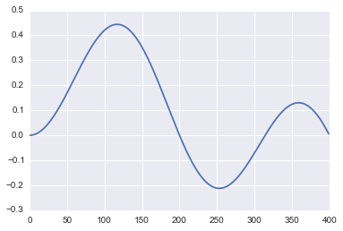

Noisy data

Now, let us add some Gaussian noise about the true data

corr=ex+0.05*np.random.normal(0,1,n)

This is how the corrupted signal looks like.

plt.plot(corr);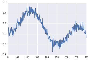

The optimization problem

Constraints

1. We want the cleaned data to be as close to the corrupted data
2. We want the successive entries in the cleaned data to be as close as possible

Mathematically, we can write this as follows:

$ $

Here, \(||(x-x_{corr})||^2\) corresponds to the first constraint and ${k=1}^{n-1} (x{k+1}-x_{k})^{2} $ corresponds to the second constraint.

Formulation as least squares problem

For the least squares problem, we would like a form of \(Ax=b\)

First constraint

Looking at the first constraint, \(||(x-x_{corr})||^2\), this can be expanded as follows:

$ (x_1 -x_{corr}(1))^2 + (x_2 -x_{corr}(2))^2 + ..(x_n -x_{corr}(n))^2$

which we can rewrite as :

$ ([1,0,0 ..0][x_1, x_2,..x_n]^T - x_{corr}(1))^2 + ([0,1,0 ..0][x_1, x_2,..x_n]^T - x_{corr}(2))^2 + …([0,0,0 ..n][x_1, x_2,..x_n]^T - x_{corr}(n))^2$

Comparing with the standard least squares, we get

\(A_{first} = I^{nxn}\) and \(b_{first} = x_{corr}\)

Second constraint

For the second constraint, \(\mu\sum_{k=1}^{n-1} (x_{k+1}-x_{k})^{2}\)

This can be written as: \((\sqrt{\mu}(x_2-x_1))^2 + (\sqrt{\mu}(x_3-x_2))^2 + .. (\sqrt{\mu}(x_n-x_{n-1}))^2\) which we can write as:

\((\sqrt{\mu}[-1,1,0,0,0,0..][x_1,x_2,..x_n]^T - 0)^2 + ...(\sqrt{\mu}[0,0,0,..,-1,1][x_1,x_2,..x_n]^T - 0)^2\)

From this formulation, we get for this constraint, \(A_{second}\) as follows (we ignore \(\sqrt{\mu}\) for now)

[-1, 1, 0, ...., 0]

[0, -1, 1, ......0]

..

[0, 0, ..... -1, 1]

and \(b_{second}\) as a zeros matrix of size (n-1, n)

Combining both constraints

So, we combine the two sets of As and bs in a bigger matrix to get \(A_{combined}\) and \(b_{combined}\) as follows:

\(A_{combined}\)

[A_first
A_second]

and \(b_{combined}\) as :

[b_first
b_second]

Constructing \(A_{second}\) matrix with parameter \(n\) and \(\mu\)

root_mu=10

d1=np.eye(n-1,n)

d1

array([[ 1.,  0.,  0., ...,  0.,  0.,  0.],
       [ 0.,  1.,  0., ...,  0.,  0.,  0.],
       [ 0.,  0.,  1., ...,  0.,  0.,  0.],
       ..., 
       [ 0.,  0.,  0., ...,  0.,  0.,  0.],
       [ 0.,  0.,  0., ...,  1.,  0.,  0.],
       [ 0.,  0.,  0., ...,  0.,  1.,  0.]])

d1=np.roll(d1,1)

d1

array([[ 0.,  1.,  0., ...,  0.,  0.,  0.],
       [ 0.,  0.,  1., ...,  0.,  0.,  0.],
       [ 0.,  0.,  0., ...,  0.,  0.,  0.],
       ..., 
       [ 0.,  0.,  0., ...,  1.,  0.,  0.],
       [ 0.,  0.,  0., ...,  0.,  1.,  0.],
       [ 0.,  0.,  0., ...,  0.,  0.,  1.]])

d2=-np.eye(n-1,n)

a_second=  root_mu*(d1+d2)

a_second

array([[-10.,  10.,   0., ...,   0.,   0.,   0.],
       [  0., -10.,  10., ...,   0.,   0.,   0.],
       [  0.,   0., -10., ...,   0.,   0.,   0.],
       ..., 
       [  0.,   0.,   0., ...,  10.,   0.,   0.],
       [  0.,   0.,   0., ..., -10.,  10.,   0.],
       [  0.,   0.,   0., ...,   0., -10.,  10.]])

Constructing \(A_{first}\) matrix with parameter \(n\)

a_first=np.eye(n)

a_first

array([[ 1.,  0.,  0., ...,  0.,  0.,  0.],
       [ 0.,  1.,  0., ...,  0.,  0.,  0.],
       [ 0.,  0.,  1., ...,  0.,  0.,  0.],
       ..., 
       [ 0.,  0.,  0., ...,  1.,  0.,  0.],
       [ 0.,  0.,  0., ...,  0.,  1.,  0.],
       [ 0.,  0.,  0., ...,  0.,  0.,  1.]])

Constructing \(A\) matrix

A=np.vstack((a_first,a_second))

A

array([[  1.,   0.,   0., ...,   0.,   0.,   0.],
       [  0.,   1.,   0., ...,   0.,   0.,   0.],
       [  0.,   0.,   1., ...,   0.,   0.,   0.],
       ..., 
       [  0.,   0.,   0., ...,  10.,   0.,   0.],
       [  0.,   0.,   0., ..., -10.,  10.,   0.],
       [  0.,   0.,   0., ...,   0., -10.,  10.]])

Similarly, we construct \(b\) matrix

corr=corr.reshape((n,1))

b_2=np.zeros((n-1,1))

b=np.vstack((corr,b_2))

Let us use least squares for our denoising for \(\mu=100\)

import numpy.linalg.linalg as LA

ans = LA.lstsq(A,b)

Comparing original, noisy and denoised signal

plt.plot(corr,label='noisy',alpha=0.4)
plt.plot(ans[0],'r',linewidth=2, label='denoised')
plt.plot(ex,'g',linewidth=2, label='original')
plt.legend();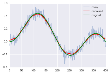

Observing the variation with \(\mu\)

Let us quickly create an interactive widget to see how denoising would be affected by different values of \(\mu\). We will view this on a log scale.

def create_A(n, mu):
    """
    Create the A matrix
    """
    d1=np.eye(n-1,n)
    d1=np.roll(d1,1)
    a_second=  np.sqrt(mu)*(d1+d2)
    a_first=np.eye(n)
    A=np.vstack((a_first,a_second))
    return A

def create_b(n):
    b_2=np.zeros((n-1,1))
    b=np.vstack((corr,b_2))
    
    return b

def denoise(mu):
    """
    Return denoised signal
    """
    n =  len(corr)
    A = create_A(n, mu)
    b = create_b(n)
    return LA.lstsq(A,b)[0]

def comparison_plot(mu):
    fig, ax = plt.subplots(figsize=(4,3))  
    ax.plot(corr,label='noisy',alpha=0.4)
    ax.plot(denoise(np.power(10,mu)),'r',linewidth=2, label='denoised')
    ax.plot(ex,'g',linewidth=2, label='original')
    plt.title(r"$\mu=%d$" % np.power(10,mu))
    plt.legend()
    return fig

from ipywidgets import StaticInteract, RangeWidget
StaticInteract(comparison_plot, mu = RangeWidget(0,5,1))    

mu:

For smaller values of \(\mu\), the first constraints is the dominant one and tries to keep the denoised signal close to the noisy one. For higher values of \(\mu\), the second constraint dominates.