Code
import autograd.numpy as np

from matplotlib import pyplot as plt
%matplotlib inline

import warnings
warnings.filterwarnings('ignore')

import GPy
In previous posts, I have talked about GP regression:
In this post, I will be talking about how to learn the parameters of a GP. I’ll keep this post simple and specific to a trivial example using RBF kernel (though the methods discussed are general.)
To keep things simple, we will assume a mean prior of zero and we will only be learning the parameters of the kernel function.
In our previous post we had mentioned (for the noiseless case):
Given train data \[ D=\left(x_{i}, y_{i}\right), i=1: N \] Given a test set \(X_{*}\) of size \(N_{*} \times d\) containing \(N_{*}\) points in \(\mathbb{R}^{d},\) we want to predict function outputs \(y_{*}\) We can write: \[ \left(\begin{array}{l} y \\ y_{*} \end{array}\right) \sim \mathcal{N}\left(\left(\begin{array}{l} \mu \\ \mu_{*} \end{array}\right),\left(\begin{array}{cc} K & K_{*} \\ K_{*}^{T} & K_{* *} \end{array}\right)\right) \] where \[ \begin{aligned} K &=\operatorname{Ker}(X, X) \in \mathbb{R}^{N \times N} \\ K_{*} &=\operatorname{Ker}\left(X, X_{*}\right) \in \mathbb{R}^{N \times N} \\ K_{* *} &=\operatorname{Ker}\left(X_{*}, X_{*}\right) \in \mathbb{R}^{N_{*} \times N_{*}} \end{aligned} \]
Thus, from the property of conditioning of multivariate Gaussian, we know that:
\[y \sim \mathcal{N}_N(\mu, K)\]
We will assume \(\mu\) to be zero. Thus, we have for the train data, the following expression:
\[y \sim \mathcal{N}_N(0, K)\]
For the noisy case, we have:
\[y \sim \mathcal{N}_N(0, K + \sigma_{noise}^2\mathcal{I}_N)\]
From this expression, we can write the log-likelihood of data computed over the kernel parameters \(\theta\) as:
\[\mathcal{LL}(\theta) = \log(\frac{\exp((-1/2)(y-0)^T (K+\sigma_{noise}^2\mathcal{I}_N)^{-1}(y-0))}{(2\pi)^{N/2}|(K+\sigma_{noise}^2\mathcal{I}_N)|^{1/2}})\]
Thus, we can write:
\[\mathcal{LL}(\theta) =\log P(\mathbf{y} | X, \theta)=-\frac{1}{2} \mathbf{y}^{\top} M^{-1} \mathbf{y}-\frac{1}{2} \log |M|-\frac{N}{2} \log 2 \pi\]
where \[M = K + \sigma_{noise}^2\mathcal{I}_N\]
As before, we will be using the excellent Autograd library for automatically computing the gradient of an objective function with respect to the parameters. We will also be using GPy for verifying our calculations.
Let us start with some basic imports.
import autograd.numpy as np
from matplotlib import pyplot as plt
%matplotlib inline
import warnings
warnings.filterwarnings('ignore')
import GPyThe definition of the (1-dimensional) RBF kernel has a Gaussian-form, defined as:
\[ \kappa_\mathrm{rbf}(x_1,x_2) = \sigma^2\exp\left(-\frac{(x_1-x_2)^2}{2\mathscr{l}^2}\right) \]
def rbf(x1, x2, sigma, l):
return (sigma**2)*(np.exp(-(x1-x2)**2/(2*(l**2)))) # Create a 1-D RBF kernel with default parameters
k = GPy.kern.RBF(1)
# Preview the kernel's parameters
k| rbf. | value | constraints | priors |
|---|---|---|---|
| variance | 1.0 | +ve | |
| lengthscale | 1.0 | +ve |
rbf(1, 0, 1, 1)==k.K(np.array([[1]]), np.array([[0]])).flatten()array([ True])Looks good. Our function is matching GPy’s kernel.
# lambda function, call f(x) to generate data
f = lambda x: 0.4*x**2 - 0.15*x**3 + 0.5*x**2 - 0.002*x**5 + 0.0002*x**6 +0.5*(x-2)**2
n = 20
np.random.seed(0)
X = np.linspace(0.05, 4.95, n)[:,None]
Y = f(X) + np.random.normal(0., 0.1, (n,1)) # note that np.random.normal takes mean and s.d. (not variance), 0.1^2 = 0.01
plt.plot(X, Y, "kx", mew=2, label='Train points')
plt.xlabel("x"), plt.ylabel("f")
plt.legend();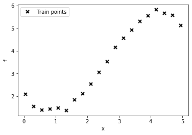
Based on our above mentioned theory, we can now write the NLL function as follows
def nll(sigma=1, l=1, noise_std=1):
    n = X.shape[0]
    cov = rbf(X, X.T, sigma, l) + (noise_std**2)*np.eye(X.shape[0])
    nll_ar =  0.5*(Y.T@np.linalg.inv(cov)@Y) + 0.5*n*np.log(2*np.pi) + 0.5*np.log(np.linalg.det(cov))
return nll_ar[0,0]We will now compare the NLL from our method with GPy for a fixed set of parameters
nll(1, 1, 1)40.103960984801276k.lengthscale = 1
k.variance = 1
m = GPy.models.GPRegression(X, Y, k, normalizer=False)
m.Gaussian_noise = 1
print(m)Name : GP regression Objective : 40.103961039553916 Number of Parameters : 3 Number of Optimization Parameters : 3 Updates : True Parameters: GP_regression. | value | constraints | priors rbf.variance | 1.0 | +ve | rbf.lengthscale | 1.0 | +ve | Gaussian_noise.variance | 1.0 | +ve |
Excellent, we can see that our method gives the same NLL. Looks like we are on the right track! One caveat here is that I have set the normalizer to be False, which means that GPy will not be mean centering the data.
We will now use GPy to optimize the GP parameters
m = GPy.models.GPRegression(X, Y, k, normalizer=False)
m.optimize()
print(m)
Name : GP regression Objective : -2.9419881541130053 Number of Parameters : 3 Number of Optimization Parameters : 3 Updates : True Parameters: GP_regression. | value | constraints | priors rbf.variance | 27.837243180547883 | +ve | rbf.lengthscale | 2.732180018958835 | +ve | Gaussian_noise.variance | 0.007573211752763481 | +ve |
It seems that variance close to 28 and length scale close to 2.7 give the optimum objective for the GP
We will now plot the NLL obtained from our calculations as a function of variance and lengthscale. For comparing our solution with GPy solution, I will be setting noise variance to be 0.0075
import numpy as numpy
x_grid_2, y_grid_2 = numpy.mgrid[0.1:6:0.04, 0.1:4:0.03]

li = np.zeros_like(x_grid_2)
for i in range(x_grid_2.shape[0]):
    for j in range(x_grid_2.shape[1]):
li[i, j] = nll(x_grid_2[i, j], y_grid_2[i, j], np.sqrt(.007573211752763481))plt.contourf(x_grid_2, y_grid_2, li)
plt.gca().set_aspect('equal')
plt.xlabel(r"$\sigma$")
plt.ylabel(r"$l$")
plt.colorbar()
plt.title(r"NLL ($\sigma, l$)")Text(0.5, 1.0, 'NLL ($\\sigma, l$)')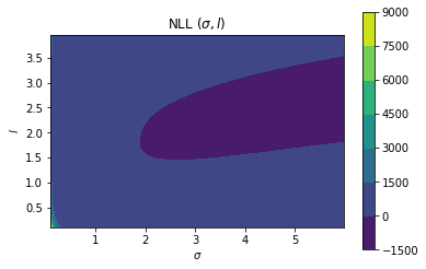
We will now try to find the “optimum” \(\sigma\) and lengthscale from this NLL space.
print(li.min())
aa, bb = np.unravel_index(li.argmin(), li.shape)
print(x_grid_2[aa, 0]**2, y_grid_2[bb, 0])
-2.9418973674348727
28.09 0.1Excellent, it looks like we are pretty close to the optimum NLL as reported by GPy and our parameters learnt are also pretty similar. But, we have not even done a thorough search. We will now be using gradient descent to help us find the optimum set of parameters.
from autograd import elementwise_grad as egrad
from autograd import gradgrad_objective = grad(nll, argnum=[0, 1, 2])sigma = 2.
l = 2.
noise = 1.
lr = 1e-3
num_iter = 100
nll_arr = np.zeros(num_iter)
for iteration in range(num_iter):
nll_arr[iteration] = nll(sigma, l, noise)
del_sigma, del_l, del_noise = grad_objective(sigma, l, noise)
sigma = sigma - lr*del_sigma
l = l - lr*del_l
noise = noise - lr*del_noiseprint(sigma**2, l, noise)5.108812267877177 1.9770216805277476 0.11095385387537618plt.plot(nll_arr)
plt.xlabel("Iteration")
plt.ylabel("NLL")Text(0, 0.5, 'NLL')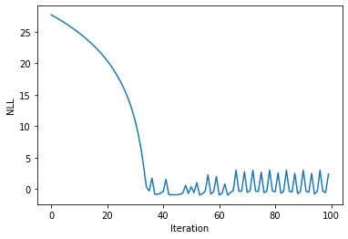
sigma = 2.
l = 2.
noise = 1.
lr = 1e-3
num_iter = 100
nll_arr = np.zeros(num_iter)
fig, ax = plt.subplots()
for iteration in range(num_iter):
    nll_arr[iteration] = nll(sigma, l, noise)
    del_sigma, del_l, del_noise = grad_objective(sigma, l, noise)
    sigma = sigma - lr*del_sigma
    l = l - lr*del_l
    noise = noise - lr*del_noise
    k.lengthscale = l
    k.variance = sigma**2
    m = GPy.models.GPRegression(X, Y, k, normalizer=False)
    m.Gaussian_noise = noise**2
    m.plot(ax=ax)['dataplot'];
    plt.ylim((0, 6))
    plt.title(f"Iteration: {iteration:04}, Objective :{nll_arr[iteration]}")
    plt.savefig(f"/home/nipunbatra-pc/Desktop/gp_learning/{iteration:04}.png")
    plt.cla();
plt.clf()
<Figure size 432x288 with 0 Axes>!convert -delay 20 -loop 0 /home/nipunbatra-pc/Desktop/gp_learning/*.png gp-learning.gif
Excellent, we can see the “learning” process over time. Our final objective is comparable to GPy’s objective.
There are a few things I have mentioned, yet have not gone into their details and I would encourage you to try those out.
There you go. Till next time!