Sampling from common distributions

import numpy as np
import matplotlib.pyplot as plt
%matplotlib inline

PRNG

Uniform distribution

I am pasting the code from vega-vis

export default function(seed) {
  // Random numbers using a Linear Congruential Generator with seed value
  // Uses glibc values from https://en.wikipedia.org/wiki/Linear_congruential_generator
  return function() {
    seed = (1103515245 * seed + 12345) % 2147483647;
    return seed / 2147483647;
  };
}

def random_gen(seed, num):
    out = np.zeros(num)
    out[0] =  (1103515245 * seed + 12345) % 2147483647
    for i in range(1, num):
        out[i] = (1103515245 * out[i-1] + 12345) % 2147483647
    return out/2147483647
        
        

plt.hist(random_gen(0, 5000), density=True, alpha=0.5, label='Our implementation');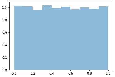

plt.hist(random_gen(0, 5000), density=True, alpha=0.5, label='Our implementation');
plt.hist(np.random.random(5000), density=True, alpha=0.4, label='Numpy implementation');
plt.legend()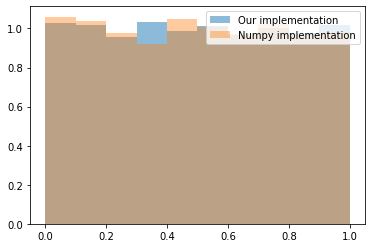

<matplotlib.legend.Legend at 0x7f51d3cbd290>

Inverse transform sampling

Exponential distribution

Borrowing from Wikipedia.

The probability density function (pdf) of an exponential distribution is \[ f(x ; \lambda)=\left\{\begin{array}{ll} \lambda e^{-\lambda x} & x \geq 0 \\ 0 & x \leq 0 \end{array}\right. \]

The exponential distribution is sometimes parametrized in terms of the scale parameter \(\beta=1 / \lambda:\) \[ f(x ; \beta)=\left\{\begin{array}{ll} \frac{1}{\beta} e^{-x / \beta} & x \geq 0 \\ 0 & x<0 \end{array}\right. \]

The cumulative distribution function is given by \[ F(x ; \lambda)=\left\{\begin{array}{ll} 1-e^{-\lambda x} & x \geq 0 \\ 0 & x<0 \end{array}\right. \]

from scipy.stats import expon
rvs = [expon(scale=s) for s in [1/1., 1/2., 1/3.]]

x = np.arange(0, 10, 0.1)
for i, lambda_val in enumerate([1, 2, 3]):
    plt.plot(x, rvs[i].pdf(x), lw=2, label=r'$\lambda=%s$' %lambda_val)
plt.legend()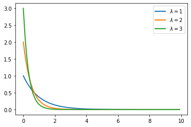

<matplotlib.legend.Legend at 0x7f51da6d4e10>

For the purposes of this notebook, I will be looking only at the standard exponential or set the scale to 1.

Let us now view the CDF of the standard exponential.

fig, ax = plt.subplots(nrows=2, sharex=True)
ax[0].plot(x, expon().pdf(x), lw=2)
ax[0].set_title("PDF")
ax[1].set_title("CDF")
ax[1].plot(x, expon().cdf(x), lw=2,)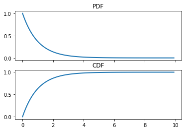

r = expon.rvs(size=1000)

plt.hist(r, normed=True, bins=100)
plt.plot(x, expon().pdf(x), lw=2)

/home/nipunbatra-pc/anaconda3/lib/python3.7/site-packages/ipykernel_launcher.py:1: MatplotlibDeprecationWarning: 
The 'normed' kwarg was deprecated in Matplotlib 2.1 and will be removed in 3.1. Use 'density' instead.
  """Entry point for launching an IPython kernel.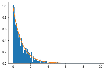

Inverse of the CDF of exponential

The cumulative distribution function is given by \[ F(x ; \lambda)=\left\{\begin{array}{ll} 1-e^{-\lambda x} & x \geq 0 \\ 0 & x<0 \end{array}\right. \]

Let us consider only \(x \geq 0\).

Let \(u = F^{-1}\) be the inverse of the CDF of \(F\).

\[ u = 1-e^{-\lambda x} \\ 1- u = e^{-\lambda x} \\ \log(1-u) = -\lambda x\\ x = -\frac{\log(1-u)}{\lambda} \]

def inverse_transform(lambda_val, num_samples):
    u = np.random.random(num_samples)
    x = -np.log(1-u)/lambda_val
    return x

plt.hist(inverse_transform(1, 5000), bins=100, normed=True,label='Generated using our function');
plt.plot(x, expon().pdf(x), lw=4, label='Generated using scipy')
plt.legend()

/home/nipunbatra-pc/anaconda3/lib/python3.7/site-packages/ipykernel_launcher.py:1: MatplotlibDeprecationWarning: 
The 'normed' kwarg was deprecated in Matplotlib 2.1 and will be removed in 3.1. Use 'density' instead.
  """Entry point for launching an IPython kernel.

<matplotlib.legend.Legend at 0x7f51d5f95410>

Drawing samples from Laplace distribution

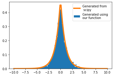
A random variable has a Laplace \((\mu, b)\) distribution if its probability density function is \[ f(x | \mu, b)=\frac{1}{2 b} \exp \left(-\frac{|x-\mu|}{b}\right) \]

\[F^{-1}(u)=\mu-b \operatorname{sgn}(u-0.5) \ln (1-2|u-0.5|)\]

def inverse_transform_laplace(b, mu, num_samples):
    u = np.random.random(num_samples)
    x = mu-b*np.sign(u-0.5)*np.log(1-2*np.abs(u-0.5))
    return x

from scipy.stats import laplace
plt.hist(inverse_transform_laplace(1, 0, 5000),bins=100, density=True, label='Generated using \nour function');
x_n = np.linspace(-10, 10, 100)
plt.plot(x_n, laplace().pdf(x_n), lw=4, label='Generated from\n scipy')
plt.legend()

<matplotlib.legend.Legend at 0x7f51d4a99750>

Box-Muller transform