Using GPy and some interactive visualisations for understanding GPR and applying on a real world data set
ML
Author
Nipun Batra
Published
June 26, 2020
Disclaimer
This blog post is forked from GPSS 2019Lab 1. This is produced only for educational purposes. All credit goes to the GPSS organisers.
Code
# Support for mathsimport numpy as np# Plotting toolsfrom matplotlib import pyplot as plt# we use the following for plotting figures in jupyter%matplotlib inlineimport warningswarnings.filterwarnings('ignore')# GPy: Gaussian processes libraryimport GPyfrom IPython.display import display
Covariance functions, aka kernels
We will define a covariance function, from hereon referred to as a kernel, using GPy. The most commonly used kernel in machine learning is the Gaussian-form radial basis function (RBF) kernel. It is also commonly referred to as the exponentiated quadratic or squared exponential kernel – all are equivalent.
The definition of the (1-dimensional) RBF kernel has a Gaussian-form, defined as:
It has two parameters, described as the variance, \(\sigma^2\) and the lengthscale \(\mathscr{l}\).
In GPy, we define our kernels using the input dimension as the first argument, in the simplest case input_dim=1 for 1-dimensional regression. We can also explicitly define the parameters, but for now we will use the default values:
Code
# Create a 1-D RBF kernel with default parametersk = GPy.kern.RBF(lengthscale=0.5, input_dim=1, variance=4)# Preview the kernel's parametersk
rbf.
value
constraints
priors
variance
4.0
+ve
lengthscale
0.5
+ve
Code
fig, ax = plt.subplots()from matplotlib.animation import FuncAnimationfrom matplotlib import rcls = [0.0005, 0.05, 0.25, 0.5, 1., 2., 4.]X = np.linspace(0.,1.,500)# 500 points evenly spaced over [0,1]X = X[:,None]mu = np.zeros((500))def update(iteration): ax.cla() k = GPy.kern.RBF(1) k.lengthscale = ls[iteration]# Calculate the new covariance function at k(x,0) C = k.K(X,X) Z = np.random.multivariate_normal(mu,C,40)for i inrange(40): ax.plot(X[:],Z[i,:],color='k',alpha=0.2) ax.set_title("$\kappa_{rbf}(x,x')$\nLength scale = %s"%k.lengthscale[0]); ax.set_ylim((-4, 4))num_iterations =len(ls)anim = FuncAnimation(fig, update, frames=np.arange(0, num_iterations-1, 1), interval=500)plt.close()rc('animation', html='jshtml')anim
In the animation above, as you increase the length scale, the learnt functions keep getting smoother.
Code
fig, ax = plt.subplots()from matplotlib.animation import FuncAnimationfrom matplotlib import rcvar = [0.0005, 0.05, 0.25, 0.5, 1., 2., 4., 9.]X = np.linspace(0.,1.,500)# 500 points evenly spaced over [0,1]X = X[:,None]mu = np.zeros((500))def update(iteration): ax.cla() k = GPy.kern.RBF(1) k.variance = var[iteration]# Calculate the new covariance function at k(x,0) C = k.K(X,X) Z = np.random.multivariate_normal(mu,C,40)for i inrange(40): ax.plot(X[:],Z[i,:],color='k',alpha=0.2) ax.set_title("$\kappa_{rbf}(x,x')$\nVariance = %s"%k.variance[0]); ax.set_ylim((-4, 4))num_iterations =len(ls)anim = FuncAnimation(fig, update, frames=np.arange(0, num_iterations-1, 1), interval=500)plt.close()rc('animation', html='jshtml')anim
In the animation above, as you increase the variance, the scale of values increases.
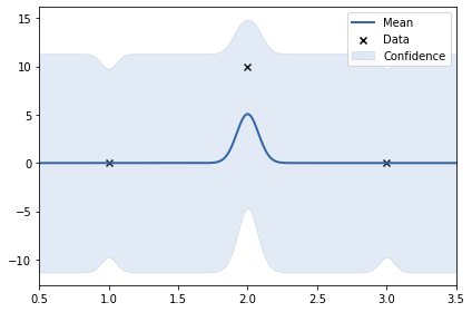
In the above example, the y values are: 0, 10, 0. The data set is not smooth. Thus, length scale learnt uis very small (0.24). Noise variance of RBF kernel also increased to accomodate the 10.
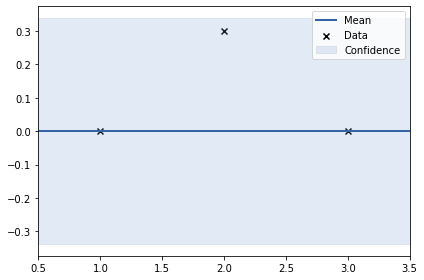
In the above examples, the y values are: 0, 0.3, 0. The data set is the smoothest amongst the four. Thus, length scale learnt is large (2.1). Noise variance of RBF kernel is also small.