Learning Gaussian Process regression parameters using mini-batch stochastic gradient descent

Defining log-likelihood

In our previous post we had mentioned (for the noiseless case):

Given train data \[ D=\left(x_{i}, y_{i}\right), i=1: N \] Given a test set \(X_{*}\) of size \(N_{*} \times d\) containing \(N_{*}\) points in \(\mathbb{R}^{d},\) we want to predict function outputs \(y_{*}\) We can write: \[ \left(\begin{array}{l} y \\ y_{*} \end{array}\right) \sim \mathcal{N}\left(\left(\begin{array}{l} \mu \\ \mu_{*} \end{array}\right),\left(\begin{array}{cc} K & K_{*} \\ K_{*}^{T} & K_{* *} \end{array}\right)\right) \] where \[ \begin{aligned} K &=\operatorname{Ker}(X, X) \in \mathbb{R}^{N \times N} \\ K_{*} &=\operatorname{Ker}\left(X, X_{*}\right) \in \mathbb{R}^{N \times N} \\ K_{* *} &=\operatorname{Ker}\left(X_{*}, X_{*}\right) \in \mathbb{R}^{N_{*} \times N_{*}} \end{aligned} \]

Thus, from the property of conditioning of multivariate Gaussian, we know that:

\[y \sim \mathcal{N}_N(\mu, K)\]

We will assume \(\mu\) to be zero. Thus, we have for the train data, the following expression:

\[y \sim \mathcal{N}_N(0, K)\]

For the noisy case, we have:

\[y \sim \mathcal{N}_N(0, K + \sigma_{noise}^2\mathcal{I}_N)\]

From this expression, we can write the log-likelihood of data computed over the kernel parameters \(\theta\) as:

\[\mathcal{LL}(\theta) = \log(\frac{\exp((-1/2)(y-0)^T (K+\sigma_{noise}^2\mathcal{I}_N)^{-1}(y-0))}{(2\pi)^{N/2}|(K+\sigma_{noise}^2\mathcal{I}_N)|^{1/2}})\]

Thus, we can write:

\[\mathcal{LL}(\theta) =\log P(\mathbf{y} | X, \theta)=-\frac{1}{2} \mathbf{y}^{\top} M^{-1} \mathbf{y}-\frac{1}{2} \log |M|-\frac{N}{2} \log 2 \pi\]

where \[M = K + \sigma_{noise}^2\mathcal{I}_N\]

Imports

As before, we will be using the excellent Autograd library for automatically computing the gradient of an objective function with respect to the parameters. We will also be using GPy for verifying our calculations.

Let us start with some basic imports.

Code

import autograd.numpy as np

from matplotlib import pyplot as plt
%matplotlib inline

import warnings
warnings.filterwarnings('ignore')

import GPy

Defining our RBF kernel

The definition of the (1-dimensional) RBF kernel has a Gaussian-form, defined as:

\[ \kappa_\mathrm{rbf}(x_1,x_2) = \sigma^2\exp\left(-\frac{(x_1-x_2)^2}{2\mathscr{l}^2}\right) \]

Code

def rbf(x1, x2, sigma, l):
    return (sigma**2)*(np.exp(-(x1-x2)**2/(2*(l**2))))

Defining GPy’s RBF kernel

Code

# Create a 1-D RBF kernel with default parameters
k = GPy.kern.RBF(1)
# Preview the kernel's parameters
k

rbf.	value	constraints	priors
variance	1.0	+ve
lengthscale	1.0	+ve

Matching our RBF kernel with GPy’s kernel

Code

rbf(1, 0, 1, 1)==k.K(np.array([[1]]), np.array([[0]])).flatten()

array([ True])

Looks good. Our function is matching GPy’s kernel.

GP Regresion

Creating a data set

Code

# lambda function, call f(x) to generate data
f = lambda x: 0.4*x**2 - 0.15*x**3 + 0.5*x**2 - 0.002*x**5 + 0.0002*x**6 +0.5*(x-2)**2
n = 50
np.random.seed(0)
X = np.linspace(0.05, 4.95, n)[:,None]
Y = f(X) + np.random.normal(0., 0.1, (n,1)) # note that np.random.normal takes mean and s.d. (not variance), 0.1^2 = 0.01
plt.plot(X, Y, "kx", mew=0.5, label='Train points')
plt.xlabel("x"), plt.ylabel("f")
plt.legend();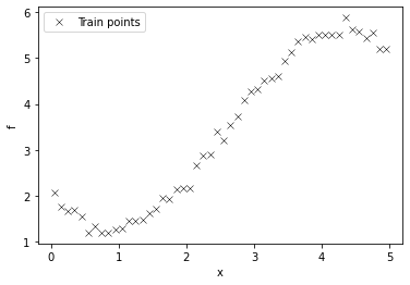

Function to compute negative log likelihood

Based on our above mentioned theory, we can now write the NLL function as follows

Code

def nll(X, Y, sigma, l, noise_std):
    n = X.shape[0]
    cov = rbf(X, X.T, sigma, l) + (noise_std**2)*np.eye(X.shape[0])
    nll_ar =  0.5*(Y.T@np.linalg.inv(cov)@Y) + 0.5*n*np.log(2*np.pi) + 0.5*np.log(np.linalg.det(cov)) 
    return nll_ar[0,0]

Comparing the NLL from our method with the NLL from GPy

We will now compare the NLL from our method with GPy for a fixed set of parameters

Code

nll(X,Y, 1, 1, 1)

70.9892893011209

Code

k.lengthscale = 1
k.variance = 1
m = GPy.models.GPRegression(X, Y, k, normalizer=False)
m.Gaussian_noise = 1
print(m)

Name : GP regression

Objective : 70.98928950981251

Number of Parameters : 3

Number of Optimization Parameters : 3

Updates : True

Parameters:

  GP_regression.           |  value  |  constraints  |  priors

  rbf.variance             |    1.0  |      +ve      |        

  rbf.lengthscale          |    1.0  |      +ve      |        

  Gaussian_noise.variance  |    1.0  |      +ve      |

Excellent, we can see that our method gives the same NLL. Looks like we are on the right track! One caveat here is that I have set the normalizer to be False, which means that GPy will not be mean centering the data.

Optimizing the GP using GPy

We will now use GPy to optimize the GP parameters

Code

m = GPy.models.GPRegression(X, Y, k, normalizer=False)
m.optimize()
print(m)

Name : GP regression

Objective : -20.145595097323056

Number of Parameters : 3

Number of Optimization Parameters : 3

Updates : True

Parameters:

  GP_regression.           |                 value  |  constraints  |  priors

  rbf.variance             |     38.67759006151069  |      +ve      |        

  rbf.lengthscale          |    2.9466566795409825  |      +ve      |        

  Gaussian_noise.variance  |  0.012471600151185298  |      +ve      |

It seems that variance close to 28 and length scale close to 2.7 give the optimum objective for the GP

Plotting the NLL as a function of variance and lenghtscale

We will now plot the NLL obtained from our calculations as a function of variance and lengthscale. For comparing our solution with GPy solution, I will be setting noise variance to be 0.0075

We will now try to find the “optimum” \(\sigma\) and lengthscale from this NLL space.

Code

X.shape

(50, 1)

Code

batch_size = 20
idx = np.random.randint(X.shape[0], size=batch_size)
X_subset, Y_subset = X[idx, :], Y[idx]
X_subset, Y_subset

plt.plot(X, Y, "kx", mew=2, label='Train points')

plt.plot(X_subset, Y_subset, "go", mew=2, label='Batch of Train points')

plt.legend()
plt.title("NLL =  %0.3f"  %nll(X_subset, Y_subset, 1, 1, 1))

Text(0.5, 1.0, 'NLL =  40.707')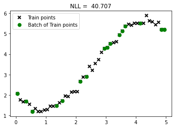

Gradient descent using autograd

Code

from autograd import elementwise_grad as egrad
from autograd import grad

Code

grad_objective = grad(nll, argnum=[2, 3, 4])

Visualising the objective as a function of iteration

Code

sigma = 2.
l = 2.
noise = 0.5
lr = 1e-2
num_iter = 1500
np.random.seed(0)
nll_arr = np.zeros(num_iter)
for iteration in range(num_iter):
    idx = np.random.randint(X.shape[0], size=batch_size)
    X_subset, Y_subset = X[idx, :], Y[idx]
     
    nll_arr[iteration] = nll(X_subset, Y_subset, sigma, l, noise)
    del_sigma, del_l, del_noise = grad_objective(X_subset, Y_subset, sigma, l, noise)
    sigma = sigma - lr*del_sigma
    l = l - lr*del_l
    noise = noise - lr*del_noise
    
    lr = lr/(iteration+1)

Code

print(sigma**2, l, noise)

4.3561278602353966 1.983897766041748 -0.10206454293334008

Code

plt.plot(nll_arr)
plt.xlabel("Iteration")
plt.ylabel("NLL")

Text(0, 0.5, 'NLL')

Choosing N-Neighbors for SGD batch

Code

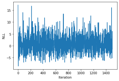
sigma = 2.
l = 2.
noise = 0.5
lr = 1e-2
num_iter = 1500
np.random.seed(0)
nll_arr = np.zeros(num_iter)
for iteration in range(num_iter):
    # Sample 1 point
    idx = np.random.randint(X.shape[0], size=1)
    x_val = X[idx]

    K = batch_size 
    a = np.abs(X - x_val).flatten()
    idx = np.argpartition(a,K)[:K] 
    X_subset = X[idx, :]
    Y_subset = Y[idx, :]
     
    nll_arr[iteration] = nll(X_subset, Y_subset, sigma, l, noise)
    del_sigma, del_l, del_noise = grad_objective(X_subset, Y_subset, sigma, l, noise)
    sigma = sigma - lr*del_sigma
    l = l - lr*del_l
    noise = noise - lr*del_noise
    
    lr = lr/(iteration+1)

Code

plt.plot(nll_arr)
plt.xlabel("Iteration")
plt.ylabel("NLL")

Text(0, 0.5, 'NLL')

Applying gradient descent and visualising the learnt function

Code

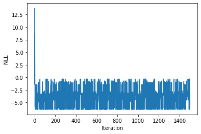
sigma = 2.
l = 2.
noise = 0.5
lr = 1e-2
num_iter = 100
batch_size = 5
nll_arr = np.zeros(num_iter)
fig, ax = plt.subplots()
np.random.seed(0)
for iteration in range(num_iter):
    # Sample 1 point
    idx = np.random.randint(X.shape[0], size=1)
    x_val = X[idx]

    K = batch_size 
    a = np.abs(X - x_val).flatten()
    idx = np.argpartition(a,K)[:K] 
    X_subset = X[idx, :]
    Y_subset = Y[idx, :]
     
    nll_arr[iteration] = nll(X_subset, Y_subset, sigma, l, noise)
    del_sigma, del_l, del_noise = grad_objective(X_subset, Y_subset, sigma, l, noise)
    sigma = sigma - lr*del_sigma
    l = l - lr*del_l
    noise = noise - lr*del_noise
    k.lengthscale = l
    k.variance = sigma**2
    m = GPy.models.GPRegression(X, Y, k, normalizer=False)
    m.Gaussian_noise = noise**2
    m.plot(ax=ax, alpha=0.2)['dataplot'];
    ax.scatter(X_subset, Y_subset, color='green', marker='*', s = 50)
    plt.ylim((0, 6))
    #plt.title(f"Iteration: {iteration:04}, Objective :{nll_arr[iteration]:04.2f}")
    plt.savefig(f"/Users/nipun/Desktop/gp_learning/{iteration:04}.png")
    ax.clear()
    lr = lr/(iteration+1)
plt.clf()

<Figure size 432x288 with 0 Axes>

Code

print(sigma**2, l, noise)

4.239252534833201 2.0031950532157596 0.30136335707188894

Code

!convert -delay 40 -loop 0 /Users/nipun/Desktop/gp_learning/*.png gp-learning-new.gif