Sampling from univariate and multivariate normal distributions using Box-Muller transform

In this notebook I’ll talk about sampling from univariate and multivariate normal distributions. I’ll mostly directly write the code and show the output. The excellent linked references provide the background.

Code

import numpy as np
import matplotlib.pyplot as plt
import tensorflow as tf
import seaborn as sns
import tensorflow_probability as tfp
import pandas as pd
tfd = tfp.distributions
tfl = tfp.layers
tfb = tfp.bijectors

sns.reset_defaults()
sns.set_context(context='talk',font_scale=1)
%matplotlib inline
%config InlineBackend.figure_format='retina'

Sampling from a univariate normal

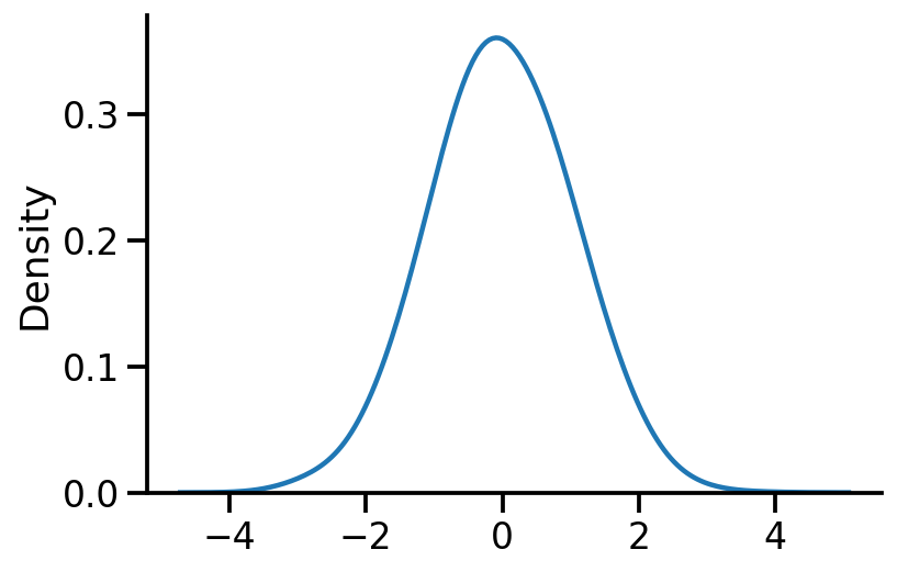
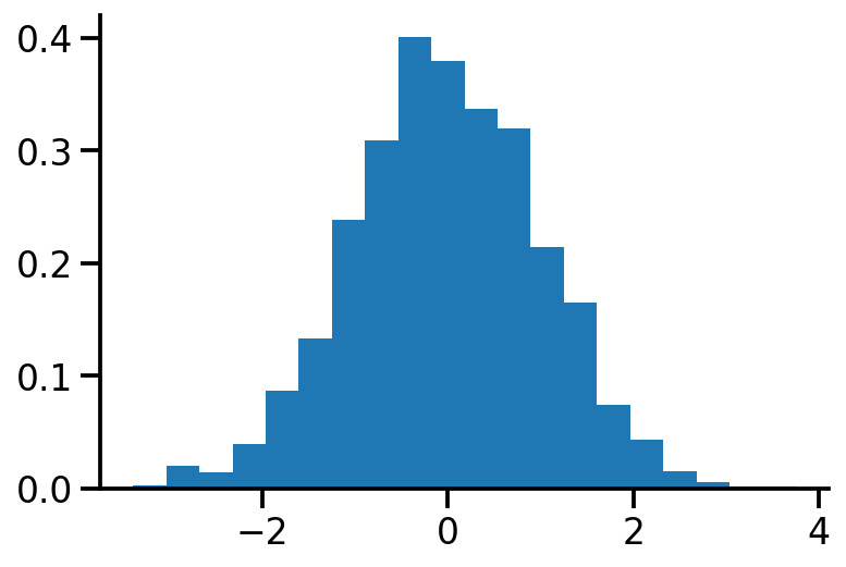
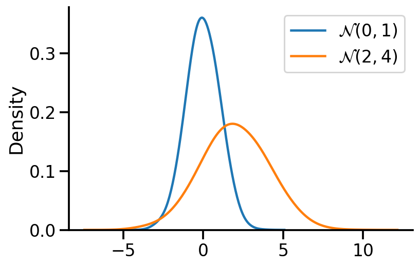
The goal here is to sample from \(\mathcal{N}(\mu, \sigma^2)\). The key idea is to use samples from a uniform distribution to first get samples for a standard normal \(\mathcal{N}(0, 1)\) and then apply an affine transformation to get samples for \(\mathcal{N}(\mu, \sigma^2)\).

Sampling from uniform distribution

Code

U = tf.random.uniform((1000, 2))
U1, U2 = U[:, 0], U[:, 1]

2022-02-04 12:00:15.559198: I tensorflow/core/platform/cpu_feature_guard.cc:151] This TensorFlow binary is optimized with oneAPI Deep Neural Network Library (oneDNN) to use the following CPU instructions in performance-critical operations:  AVX2 FMA
To enable them in other operations, rebuild TensorFlow with the appropriate compiler flags.

Applying the Box-Muller transform

Code

X1 = tf.sqrt(-2*tf.math.log(U1))*tf.cos(2*np.pi*U2)
X2 = tf.sqrt(-2*tf.math.log(U1))*tf.sin(2*np.pi*U2)

Code

X = tf.concat((X1, X2), axis=0)
X.shape

TensorShape([2000])

Plotting the obtained standard normal

Code

sns.kdeplot(X, bw_adjust=2)
sns.despine()

Code

plt.hist(X.numpy(), bins=20, density=True)
sns.despine()

Sampling from \(\mathcal{N}(\mu, \sigma^2)\)

We apply the affine transformation.

\(X \sim \mathcal{N}(0, 1)\)

\(Y \sim \mathcal{N}(\mu, \sigma^2)\) is equivalent to \(Y \sim \mu + \sigma X\)

Code

mu = 2.
sigma = 2.
Y = mu + sigma*X

Code

ax = sns.kdeplot(X, label=r'$\mathcal{N}(0, 1)$', bw_adjust=2)
sns.kdeplot(Y, label=r'$\mathcal{N}(2, 4)$', bw_adjust=2)
sns.despine()
plt.legend()

Sampling from multivariate normal

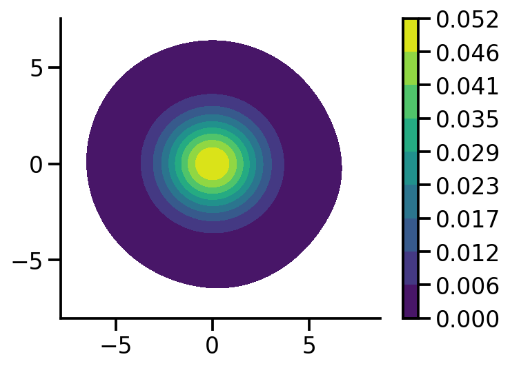
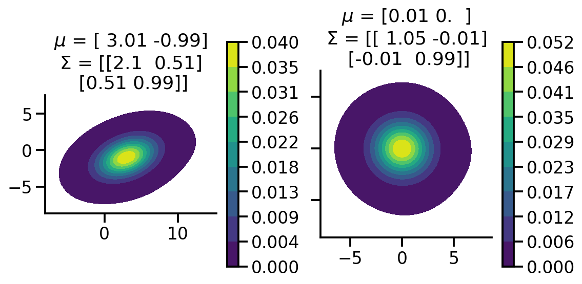
Like before, we first sample from standard multivariate normal and then apply an affine transformation to get for our desired multivariate normal.

The important thing to note in the generation of the standard multivariate normal samples is that the individial random variables are independent of each other given the identity covariance matrix. Thus, we can independently generate the samples for individual random variable.

Code

U_2D_Samples = tf.random.uniform((2, 1000, 2))

Code

U11, U12, U21, U22 = U_2D_Samples[0, :, 0], U_2D_Samples[0, :, 1],U_2D_Samples[1, :, 0],U_2D_Samples[1, :, 1]

Code

def generate(U1, U2):
    X1 = tf.sqrt(-2*tf.math.log(U1))*tf.cos(2*np.pi*U2)
    X2 = tf.sqrt(-2*tf.math.log(U1))*tf.sin(2*np.pi*U2)
    X = tf.concat((X1, X2), axis=0)
    return X

Code

X_1 = tf.reshape(generate(U11, U12), (-1, 1))
X_2 = tf.reshape(generate(U21, U22), (-1, 1))

Code

X = tf.concat((X_1, X_2), axis=1)

Code

<tf.Tensor: shape=(2000, 2), dtype=float32, numpy=
array([[-1.2652589 , -1.4106055 ],
       [ 0.09925841, -0.12048604],
       [ 0.73987466,  1.8815755 ],
       ...,
       [-0.05203251,  1.1814289 ],
       [-0.04060707, -0.14595209],
       [-0.7659936 ,  1.505757  ]], dtype=float32)>

Plotting samples from generated standard 2d normal

Code

sns.kdeplot(x=X[:, 0],
            y = X[:, 1],zorder=0, n_levels=10, shade=True, 
    cbar=True, thresh=0.001, cmap='viridis',bw_adjust=5,  cbar_kws={'format': '%.3f', })

plt.gca().set_aspect('equal')
sns.despine()

Applying the affine transformation

The main difference in the 1d and multivariate case is that instead of using \(\sigma\), we use the \(L\) cholesky matrix.

Code

mean_2d = tf.constant([3., -1.])
cov = tf.constant([[2., 0.5],
                  [0.5, 1.]])

Code

L = tf.linalg.cholesky(cov)

Code

Y_2d = mean_2d + X@tf.transpose(L)

Code

Y_2d.shape

TensorShape([2000, 2])

Code

fig, ax = plt.subplots(ncols=2, sharey=True, figsize=(8, 4))
sns.kdeplot(x=Y_2d[:, 0],
            y = Y_2d[:, 1],zorder=0, n_levels=10, shade=True, 
    cbar=True, thresh=0.001, cmap='viridis',bw_adjust=5, ax=ax[0], cbar_kws={'format': '%.3f', })

sns.kdeplot(x=X[:, 0],
            y = X[:, 1],zorder=0, n_levels=10, shade=True, 
    cbar=True, thresh=0.001, cmap='viridis',bw_adjust=5, ax=ax[1], cbar_kws={'format': '%.3f', })

ax[0].set_aspect('equal')
ax[1].set_aspect('equal')

sample_mean_tr = tf.reduce_mean(Y_2d, axis=0).numpy()
sample_mean_tr_rounded  = np.around(sample_mean_tr, 2)

cov_tr = tfp.stats.covariance(Y_2d).numpy()
cov_tr_rounded =np.around(cov_tr, 2)


sample_mean = tf.reduce_mean(X, axis=0).numpy()
sample_mean_rounded  = np.around(sample_mean, 2)

cov = tfp.stats.covariance(X).numpy()
cov_rounded =np.around(cov, 2)


ax[0].set_title(fr"$\mu$ = {sample_mean_tr_rounded}"+"\n"+ fr"$\Sigma$ = {cov_tr_rounded}")
ax[1].set_title(fr"$\mu$ = {sample_mean_rounded}"+"\n"+ fr"$\Sigma$ = {cov_rounded}")



sns.despine()
fig.tight_layout()

References

https://www.youtube.com/watch?v=DSWM7-9gK7s&list=PLISXH-iEM4Jm5B_J9p1oUNGDAUeCFZLkJ&index=38
https://www.youtube.com/watch?v=4fVQrH65aWU
https://en.wikipedia.org/wiki/Box–Muller_transform
https://en.wikipedia.org/wiki/Affine_transformation