Coin Toss (MLE, MAP, Fully Bayesian) in TF Probability

Goals

We will be studying the problem of coin tosses. I will not go into derivations but mostly deal with automatic gradient computation in TF Probability.

We have the following goals in this tutorial.

Goal 1: Maximum Likelihood Estimate (MLE)

Given a set of N observations, estimate the probability of H (denoted as \(\theta = p(H)\))

Goal 2: Maximum A-Posteriori (MAP)

Given a set of N observations and some prior knowledge on the distribution of \(\theta\), estimate the best point estimate of \(\theta\) once we have observed the dataset.

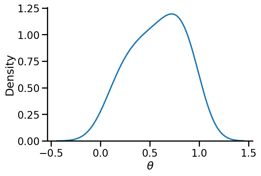
Goal 3: Fully Bayesian

Given a set of N observations and some prior knowledge on the distribution of \(\theta\), estimate the distribution of \(\theta\) once we have observed the dataset.

While I mention all the references below, I acknowledge Felix and his excellent repo and video playlist (Playlist 1, Playlist 2). They inspired me to create this post.

Basic Imports

Code

from silence_tensorflow import silence_tensorflow

silence_tensorflow()

import numpy as np
import matplotlib.pyplot as plt
import tensorflow as tf
import functools
import seaborn as sns
import tensorflow_probability as tfp
import pandas as pd

tfd = tfp.distributions
tfl = tfp.layers
tfb = tfp.bijectors

sns.reset_defaults()
sns.set_context(context="talk", font_scale=1)
%matplotlib inline
%config InlineBackend.figure_format='retina'

Creating a dataset

Let us create a dataset. We will assume the coin toss to be given as per the Bernoulli distribution. We will assume that \(\theta = p(H) = 0.75\) and generate 10 samples. We will fix the random seeds for reproducibility.

We will be encoding Heads as 1 and Tails as 0.

Code

np.random.seed(0)
tf.random.set_seed(0)

Code

distribution = tfd.Bernoulli(probs=0.75)

dataset_10 = distribution.sample(10)
print(dataset_10.numpy())
mle_estimate_10 = tf.reduce_mean(tf.cast(dataset_10, tf.float32))
tf.print(mle_estimate_10)

[0 0 0 1 1 1 1 1 0 1]
0.6

MLE

Obtaining MLE analytically

From the above 10 samples, we obtain 6 Heads (1) and 4 Tails. As per the principal of MLE, the best estimate for \(\theta = p(H) = \dfrac{n_h}{n_h+n_t} = 0.6\)

We may also notice that the value of 0.6 is far from the 0.75 value we had initially set. This is possible as our dataset is small.

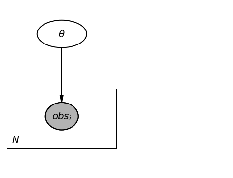
We will now verify if we get the same result using TFP. But, first, we can create a graphical model for our problem.

Graphical model

Code

import daft

pgm = daft.PGM([4, 3], origin=[0, 0])
pgm.add_node(daft.Node("theta", r"$\theta$", 1, 2.5, aspect=1.8))

pgm.add_node(daft.Node("obs", r"$obs_i$", 1, 1, aspect=1.2, observed=True))

pgm.add_edge("theta", "obs")
pgm.add_plate([0, 0.5, 2, 1.0], label=r"$N$", shift=-0.1)
pgm.render()

Obtaining MLE analytically for different dataset sizes

Code

dataset_large = distribution.sample(100000)

mle_estimate = {}
for dataset_size in [10, 50, 100, 500, 1000, 10000, 100000]:
    mle_estimate[dataset_size] = tf.reduce_mean(
        tf.cast(dataset_large[:dataset_size], tf.float32)
    )
tf.print(mle_estimate)

{10: 0.9,
 50: 0.76,
 100: 0.71,
 500: 0.746,
 1000: 0.749,
 10000: 0.749,
 100000: 0.75144}

As we can see above, when we use larger dataset sizes, our estimate matches the value we set (0.75).

Using TFP for MLE

Model setup

Code

theta = tf.Variable(0.1)
fit = tfd.Bernoulli(probs=theta)

fit.log_prob(dataset_10)

<tf.Tensor: shape=(10,), dtype=float32, numpy=
array([-0.10536052, -0.10536052, -0.10536052, -2.3025851 , -2.3025851 ,
       -2.3025851 , -2.3025851 , -2.3025851 , -0.10536052, -2.3025851 ],
      dtype=float32)>

Defining loss

We now define the negative log likelihood as our loss function and work towards minimizing it.

Code

dataset = dataset_10


def loss():
    return -tf.reduce_sum(fit.log_prob(dataset))

Tracing variables over training

Code

trace_fn = lambda traceable_quantities: {
    "loss": traceable_quantities.loss,
    "theta": theta,
}

num_steps = 150

Minimizing the loss function

Code

trace = tfp.math.minimize(
    loss_fn=loss,
    num_steps=num_steps,
    optimizer=tf.optimizers.Adam(learning_rate=0.01),
    trace_fn=trace_fn,
)

Code

theta

<tf.Variable 'Variable:0' shape=() dtype=float32, numpy=0.5981374>

Code

fig, ax = plt.subplots(nrows=2, sharex=True, figsize=(6, 4))
ax[0].plot(range(num_steps), trace["loss"])
ax[1].plot(range(num_steps), trace["theta"])
sns.despine()
ax[1].set_xlabel("Iterations")
ax[0].set_ylabel("Loss")
ax[1].set_ylabel(r"$\theta$")
fig.tight_layout()

From the above calculations, we can see that we have obtained the same estimate of ~0.6 using TFP.

Alternate way to minimize

Previously, we used the tf.math.minimize, but we can also use tf.GradientTape() for the same purpose.

Code

@tf.function
def loss_and_grads(fit):
    with tf.GradientTape() as tape:
        loss = -tf.reduce_sum(fit.log_prob(dataset))
    return loss, tape.gradient(loss, fit.trainable_variables)


optimizer = tf.keras.optimizers.Adam(learning_rate=0.01)


theta = tf.Variable(0.1)
fit = tfd.Bernoulli(probs=theta)


for i in range(num_steps):
    loss, grads = loss_and_grads(fit)
    optimizer.apply_gradients(zip(grads, fit.trainable_variables))

Code

fit.trainable_variables

(<tf.Variable 'Variable:0' shape=() dtype=float32, numpy=0.5981374>,)

We can see that we obtain the same estimate.

MAP

We will now be setting a prior over \(\theta\). A general graphical model is shown below.

Code

pgm = daft.PGM([4, 4], origin=[0, 0])
pgm.add_node(daft.Node("alpha", r"$\alpha$", 0.5, 3.5, aspect=1.8))
pgm.add_node(daft.Node("beta", r"$\beta$", 1.5, 3.5, aspect=1.8))


pgm.add_node(daft.Node("theta", r"$\theta$", 1, 2.5, aspect=2))
# pgm.add_node(daft.Node("theta", r"$\theta\sim Beta (\alpha, \beta)$", 1, 2.5, aspect=4))

pgm.add_node(daft.Node("obs", r"$obs_i$", 1, 1, aspect=1.2, observed=True))

pgm.add_edge("theta", "obs")
pgm.add_edge("alpha", "theta")
pgm.add_edge("beta", "theta")


pgm.add_plate([0, 0.5, 2, 1.0], label=r"$N$", shift=-0.1)
pgm.render()

MAP with uniform prior

First, we see the estimate for \(\theta\) if we use the uniform prior. We should obtain the MLE answer.

Code

def coin_toss_uniform_model():
    theta = yield tfp.distributions.Uniform(low=0.0, high=1.0, name="Theta")
    coin = yield tfp.distributions.Bernoulli(probs=tf.ones(100) * theta, name="Coin")

Code

coin_toss_uniform_model

<function __main__.coin_toss_uniform_model()>

Code

model_joint_uniform = tfp.distributions.JointDistributionCoroutineAutoBatched(
    lambda: coin_toss_uniform_model(), name="Original"
)

Code

model_joint_uniform

<tfp.distributions.JointDistributionCoroutineAutoBatched 'Original' batch_shape=[] event_shape=StructTuple(
  Theta=[],
  Coin=[100]
) dtype=StructTuple(
  Theta=float32,
  Coin=int32
)>

Code

def uniform_model(dataset):
    num_datapoints = len(dataset)
    theta = yield tfp.distributions.Uniform(low=0.0, high=1.0, name="Theta")

    coin = yield tfp.distributions.Bernoulli(
        probs=tf.ones(num_datapoints) * theta, name="Coin"
    )

Code

concrete_uniform_model = functools.partial(uniform_model, dataset=dataset_10)

model = tfd.JointDistributionCoroutineAutoBatched(concrete_uniform_model)

Code

model.sample()

StructTuple(
  Theta=<tf.Tensor: shape=(), dtype=float32, numpy=0.5930122>,
  Coin=<tf.Tensor: shape=(10,), dtype=int32, numpy=array([1, 0, 1, 0, 1, 1, 1, 0, 1, 1], dtype=int32)>
)

Code

th = tf.Variable(0.4)

target_log_prob_fn = lambda th: model.log_prob((th, dataset_10))

Code

x_s = tf.linspace(0.0, 1.0, 1000)
y_s = -target_log_prob_fn(x_s)
plt.plot(x_s, y_s)
plt.xlabel(r"$\theta$")
plt.ylabel("- Joint Log Prob \n(Unnormalized)")

sns.despine()

Code

trace = tfp.math.minimize(
    lambda: -target_log_prob_fn(th),
    optimizer=tf.optimizers.Adam(learning_rate=0.01),
    # trace_fn=trace_fn,
    num_steps=200,
)

Code

th

<tf.Variable 'Variable:0' shape=() dtype=float32, numpy=0.59999406>

Code

mle_estimate_10

<tf.Tensor: shape=(), dtype=float32, numpy=0.6>

We see above that our MAP estimate is fairly close to the MLE when we used the uniform prior.

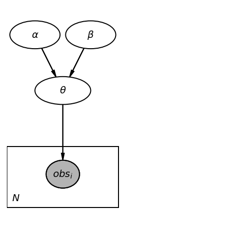
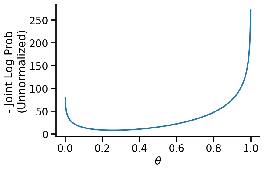
MAP with Beta prior

We will now use a much more informative prior – the Beta prior. We will be setting \(\alpha=40\) and \(\beta=10\) indicating that we have a prior belief that Tails is much more likely than Heads. This is a bad assumption and in the limited data regime will lead to poor estimates.

Code

def beta_prior_model(dataset, alpha, beta):
    num_datapoints = len(dataset)
    theta = yield tfp.distributions.Beta(
        concentration0=alpha, concentration1=beta, name="Theta"
    )

    coin = yield tfp.distributions.Bernoulli(
        probs=tf.ones(num_datapoints) * theta, name="Coin"
    )

Code

concrete_beta_prior_model_40_10 = functools.partial(
    beta_prior_model, dataset=dataset_10, alpha=40, beta=10
)

Code

model_2_40_10 = tfd.JointDistributionCoroutineAutoBatched(
    concrete_beta_prior_model_40_10
)

Code

model_2_40_10.sample()

StructTuple(
  Theta=<tf.Tensor: shape=(), dtype=float32, numpy=0.16982338>,
  Coin=<tf.Tensor: shape=(10,), dtype=int32, numpy=array([0, 0, 0, 0, 0, 0, 0, 0, 0, 0], dtype=int32)>
)

Code

model_2_40_10.prob(Theta=0.1, Coin=[0, 0, 0, 0, 0, 0, 0, 0, 1, 1])

<tf.Tensor: shape=(), dtype=float32, numpy=0.005809709>

Code

th = tf.Variable(0.2)

target_log_prob_fn = lambda th: model_2_40_10.log_prob(Theta=th, Coin=dataset_10)

Code

x_s = tf.linspace(0.0, 1.0, 1000)
y_s = -target_log_prob_fn(x_s)
plt.plot(x_s, y_s)
plt.xlabel(r"$\theta$")
plt.ylabel("- Joint Log Prob \n(Unnormalized)")

sns.despine()

Code

trace = tfp.math.minimize(
    lambda: -target_log_prob_fn(th),
    optimizer=tf.optimizers.Adam(learning_rate=0.01),
    # trace_fn=trace_fn,
    num_steps=200,
)

Code

th

<tf.Variable 'Variable:0' shape=() dtype=float32, numpy=0.25861916>

We now see that our MAP estimate for \(\theta\) is 0.25, which is very far from the MLE. Choosing a better prior would have led to better estimates. Or, if we had more data, the likelihood would have dominated over the prior resulting in better estimates.

Code

concrete_beta_prior_model_1_1 = functools.partial(
    beta_prior_model, dataset=dataset_10, alpha=1, beta=1
)

model_2_1_1 = tfd.JointDistributionCoroutineAutoBatched(concrete_beta_prior_model_1_1)

th = tf.Variable(0.2)

target_log_prob_fn = lambda th: model_2_1_1.log_prob(Theta=th, Coin=dataset_10)

trace = tfp.math.minimize(
    lambda: -target_log_prob_fn(th),
    optimizer=tf.optimizers.Adam(learning_rate=0.01),
    # trace_fn=trace_fn,
    num_steps=200,
)

th

<tf.Variable 'Variable:0' shape=() dtype=float32, numpy=0.6000196>

Our estimate for \(\theta\) is more reasonable now.

Fully Bayesian

We now need to define a model \(q(\theta)\) to act as the surrogate for our posterior \(p(\theta|D)\). Let us use a Beta distribution.

Code

q_alpha = tf.Variable(1.0)
q_beta = tf.Variable(1.0)


surrogate_posterior = tfd.Beta(concentration0=q_alpha, concentration1=q_beta, name="q")

Code

surrogate_posterior.sample()

<tf.Tensor: shape=(), dtype=float32, numpy=0.7745516>

Code

losses = tfp.vi.fit_surrogate_posterior(
    target_log_prob_fn,
    surrogate_posterior=surrogate_posterior,
    optimizer=tf.optimizers.Adam(learning_rate=0.005),
    num_steps=400,
)

Code

plt.plot(losses)
plt.xlabel("Iterations")
plt.ylabel("Loss")
sns.despine()

Code

q_alpha, q_beta

(<tf.Variable 'Variable:0' shape=() dtype=float32, numpy=1.1893775>,
 <tf.Variable 'Variable:0' shape=() dtype=float32, numpy=1.5093094>)

Code

sns.kdeplot(surrogate_posterior.sample(500).numpy(), bw_adjust=2)
sns.despine()
plt.xlabel(r"$\theta$")

Text(0.5, 0, '$\\theta$')

Generating samples on coin tosses conditioning on theta

First, let us look at the syntax and then generate 1000 samples.

Code

model_2_1_1.sample(Theta=0.1)

StructTuple(
  Theta=<tf.Tensor: shape=(), dtype=float32, numpy=0.1>,
  Coin=<tf.Tensor: shape=(10,), dtype=int32, numpy=array([1, 0, 0, 0, 0, 0, 0, 1, 0, 0], dtype=int32)>
)

Code

model_2_1_1.sample(Theta=0.9)

StructTuple(
  Theta=<tf.Tensor: shape=(), dtype=float32, numpy=0.9>,
  Coin=<tf.Tensor: shape=(10,), dtype=int32, numpy=array([1, 1, 1, 1, 1, 1, 1, 1, 1, 1], dtype=int32)>
)

We can clearly see that conditioning on r\(\theta\) changes the number of heads.

Fun check: What if we fix the dataset and sample on theta?

Code

model_2_1_1.sample(Coin=[0, 1, 1, 0, 1, 1, 1, 0])

StructTuple(
  Theta=<tf.Tensor: shape=(), dtype=float32, numpy=0.34792978>,
  Coin=<tf.Tensor: shape=(8,), dtype=int32, numpy=array([0, 1, 1, 0, 1, 1, 1, 0], dtype=int32)>
)

Code

model_2_1_1.sample(Coin=[0, 1, 1, 0, 1, 1, 1, 0])

StructTuple(
  Theta=<tf.Tensor: shape=(), dtype=float32, numpy=0.74594486>,
  Coin=<tf.Tensor: shape=(8,), dtype=int32, numpy=array([0, 1, 1, 0, 1, 1, 1, 0], dtype=int32)>
)

As we see above, we can get different \(\theta\). If our dataset was large, this effect would be less pronounced.

Code

c = model_2_1_1.sample(Theta=surrogate_posterior.sample(1000)).Coin

Code

pd.DataFrame(c)

	0	1	2	3	4	5	6	7	8	9
0	0	0	1	1	0	0	0	0	0	0
1	0	1	1	1	1	1	1	1	1	1
2	1	1	0	0	0	0	1	0	0	0
3	0	0	1	0	1	0	0	0	0	0
4	1	1	1	0	0	1	1	1	1	1
...	...	...	...	...	...	...	...	...	...	...
995	0	0	0	0	1	1	0	0	1	0
996	1	0	1	1	1	1	1	1	0	0
997	0	0	0	0	1	1	1	1	1	0
998	1	1	1	1	1	0	1	1	1	0
999	1	1	1	1	1	1	1	1	1	1

1000 rows × 10 columns

Code

sns.histplot(tf.reduce_sum(tf.cast(c, tf.float32), axis=1), bins=11)
sns.despine()

We can see the count of number of heads in 1000 samples generated from the posterior.

References (incomplete as of now)

Excellent repo and video playlist (Playlist 1, Playlist 2) by Felix
Probabilistic PCA tutorial on TFP
Discussion on joint log prob on TFP