Logistic Regression using PyTorch distributions

ML
Author

Nipun Batra

Published

February 14, 2022

Basic Imports

import numpy as np
import matplotlib.pyplot as plt
import torch
import seaborn as sns
import pandas as pd

dist =torch.distributions

sns.reset_defaults()
sns.set_context(context="talk", font_scale=1)
%matplotlib inline
%config InlineBackend.figure_format='retina'

Generative model for logistic regression

x = dist.Normal(loc = torch.tensor([0., 0.]), scale=torch.tensor([1., 2.]))
x_sample = x.sample([100])
x_sample.shape

x_dash = torch.concat((torch.ones(x_sample.shape[0], 1), x_sample), axis=1)
theta = dist.MultivariateNormal(loc = torch.tensor([0., 0., 0.]), covariance_matrix=0.5*torch.eye(3))
theta_sample = theta.sample()

p = torch.sigmoid(x_dash@theta_sample)

y = dist.Bernoulli(probs=p)
y_sample = y.sample()
plt.scatter(x_sample[:, 0], x_sample[:, 1], c = y_sample, s=40, alpha=0.5)
sns.despine()

theta_sample
tensor([ 0.6368, -0.7526,  1.4652])
from sklearn.linear_model import LogisticRegression
lr_l2 = LogisticRegression()
lr_none = LogisticRegression(penalty='none')
lr_l2.fit(x_sample, y_sample)
lr_none.fit(x_sample, y_sample)
LogisticRegression(penalty='none')
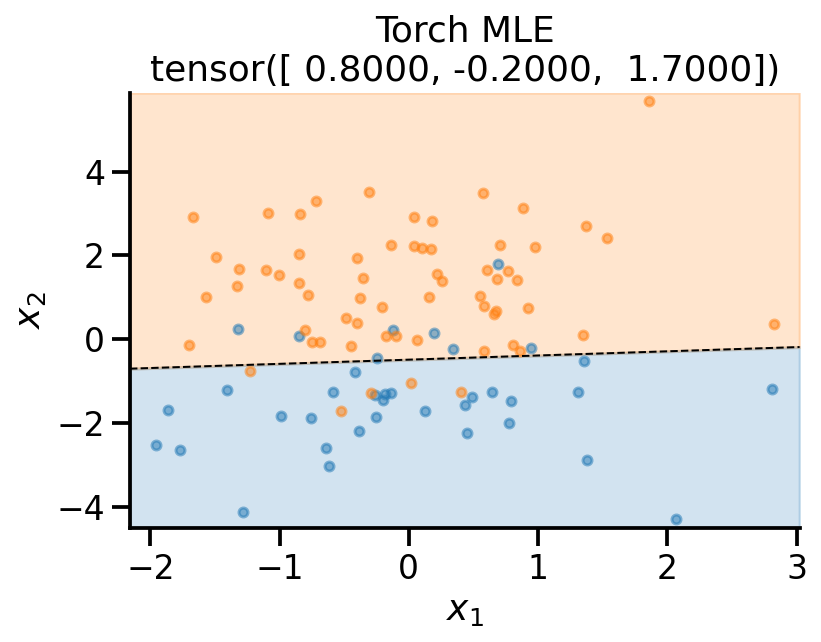
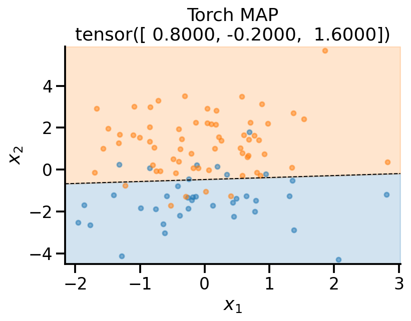
def plot_fit(x_sample, y_sample, theta, model_name):

    
    # Retrieve the model parameters.
    b = theta[0]
    w1, w2 = theta[1], theta[2]
    # Calculate the intercept and gradient of the decision boundary.
    c = -b/w2
    m = -w1/w2

    # Plot the data and the classification with the decision boundary.
    xmin, xmax = x_sample[:, 0].min()-0.2, x_sample[:, 0].max()+0.2
    ymin, ymax =  x_sample[:, 1].min()-0.2, x_sample[:, 1].max()+0.2
    xd = np.array([xmin, xmax])
    yd = m*xd + c
    plt.plot(xd, yd, 'k', lw=1, ls='--')
    plt.fill_between(xd, yd, ymin, color='tab:blue', alpha=0.2)
    plt.fill_between(xd, yd, ymax, color='tab:orange', alpha=0.2)

    plt.scatter(*x_sample[y_sample==0].T, s=20, alpha=0.5)
    plt.scatter(*x_sample[y_sample==1].T, s=20, alpha=0.5)
    plt.xlim(xmin, xmax)
    plt.ylim(ymin, ymax)
    plt.ylabel(r'$x_2$')
    plt.xlabel(r'$x_1$')
    theta_print = np.round(theta, 1)
    plt.title(f"{model_name}\n{theta_print}")
    sns.despine()
plot_fit(
    x_sample,
    y_sample,
    theta_sample,
    r"Generating $\theta$",
)

plot_fit(
    x_sample,
    y_sample,
    np.concatenate((lr_l2.intercept_.reshape(-1, 1), lr_l2.coef_), axis=1).flatten(),
    r"Sklearn $\ell_2$ penalty ",
)

plot_fit(
    x_sample,
    y_sample,
    np.concatenate((lr_none.intercept_.reshape(-1, 1), lr_none.coef_), axis=1).flatten(),
    r"Sklearn No penalty ",
)

MLE estimate PyTorch

def neg_log_likelihood(theta, x, y):
    x_dash = torch.concat((torch.ones(x.shape[0], 1), x), axis=1)
    p = torch.sigmoid(x_dash@theta)
    y_dist = dist.Bernoulli(probs=p)

    return -torch.sum(y_dist.log_prob(y))
neg_log_likelihood(theta_sample, x_sample, y_sample)
tensor(33.1907)
theta_learn_loc = torch.tensor([1., 1., 1.], requires_grad=True)
neg_log_likelihood(theta_learn_loc, x_sample, y_sample)

plot_fit(
    x_sample,
    y_sample,
    theta_learn_loc.detach(),
    r"Torch without training",
)

theta_learn_loc = torch.tensor([0., 0., 0.], requires_grad=True)
loss_array = []
loc_array = []

opt = torch.optim.Adam([theta_learn_loc], lr=0.05)
for i in range(101):
    loss_val = neg_log_likelihood(theta_learn_loc, x_sample, y_sample)
    loss_val.backward()
    loc_array.append(theta_learn_loc)
    loss_array.append(loss_val.item())

    if i % 10 == 0:
        print(
            f"Iteration: {i}, Loss: {loss_val.item():0.2f}"
        )
    opt.step()
    opt.zero_grad()
Iteration: 0, Loss: 69.31
Iteration: 10, Loss: 44.14
Iteration: 20, Loss: 35.79
Iteration: 30, Loss: 32.73
Iteration: 40, Loss: 31.67
Iteration: 50, Loss: 31.25
Iteration: 60, Loss: 31.08
Iteration: 70, Loss: 31.00
Iteration: 80, Loss: 30.97
Iteration: 90, Loss: 30.95
Iteration: 100, Loss: 30.94
plot_fit(
    x_sample,
    y_sample,
    theta_learn_loc.detach(),
    r"Torch MLE",
)

MAP estimate PyTorch

prior_theta = dist.MultivariateNormal(loc = torch.tensor([0., 0., 0.]), covariance_matrix=2*torch.eye(3))

logprob = lambda theta: -prior_theta.log_prob(theta)
theta_learn_loc = torch.tensor([0., 0., 0.], requires_grad=True)
loss_array = []
loc_array = []

opt = torch.optim.Adam([theta_learn_loc], lr=0.05)
for i in range(101):
    loss_val = neg_log_likelihood(theta_learn_loc, x_sample, y_sample) + logprob(theta_learn_loc)
    loss_val.backward()
    loc_array.append(theta_learn_loc)
    loss_array.append(loss_val.item())

    if i % 10 == 0:
        print(
            f"Iteration: {i}, Loss: {loss_val.item():0.2f}"
        )
    opt.step()
    opt.zero_grad()
Iteration: 0, Loss: 73.11
Iteration: 10, Loss: 48.06
Iteration: 20, Loss: 39.89
Iteration: 30, Loss: 37.01
Iteration: 40, Loss: 36.10
Iteration: 50, Loss: 35.78
Iteration: 60, Loss: 35.67
Iteration: 70, Loss: 35.64
Iteration: 80, Loss: 35.62
Iteration: 90, Loss: 35.62
Iteration: 100, Loss: 35.62
plot_fit(
    x_sample,
    y_sample,
    theta_learn_loc.detach(),
    r"Torch MAP",
)

References


  1. Plotting code borrwed from here: https://scipython.com/blog/plotting-the-decision-boundary-of-a-logistic-regression-model/