Code
from wand.image import Image as WImage
from wand.color import Color
img = WImage(filename='../pgm/coin-toss.pdf', resolution=300)
img.crop(0, 400, 2480, 1500)
img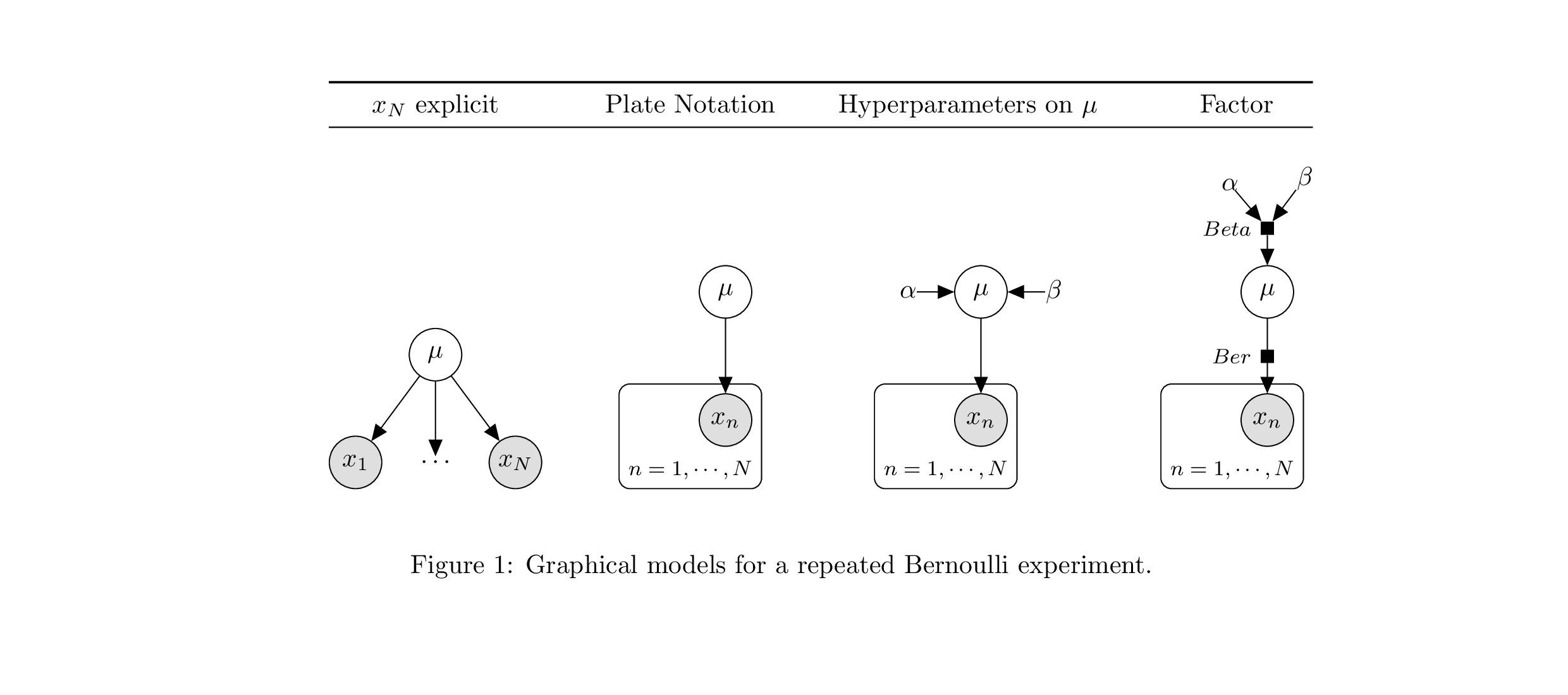
from wand.image import Image as WImage
from wand.color import Color
img = WImage(filename='../pgm/coin-toss.pdf', resolution=300)
img.crop(0, 400, 2480, 1500)
img
%cat ../pgm/coin-toss.tex\documentclass[a4paper]{article}
\usepackage{caption}
\usepackage{subcaption}
\usepackage{tikz}
\usetikzlibrary{bayesnet}
\usepackage{booktabs}
\setlength{\tabcolsep}{12pt}
\begin{document}
\begin{figure}[ht]
\begin{center}
\begin{tabular}{@{}cccc@{}}
\toprule
$x_N$ explicit & Plate Notation & Hyperparameters on $\mu$ & Factor\\ \midrule
& & & \\
\begin{tikzpicture}
\node[obs] (x1) {$x_1$};
\node[const, right=0.5cm of x1] (dots) {$\cdots$};
\node[obs, right=0.5cm of dots] (xn) {$x_N$};
\node[latent, above=of dots] (mu) {$\mathbf{\mu}$};
\edge {mu} {x1,dots,xn} ; %
\end{tikzpicture}&
\begin{tikzpicture}
\node[obs] (xn) {$x_n$};
\node[latent, above=of xn] (mu) {$\mathbf{\mu}$};
\plate{}{(xn)}{$n = 1, \cdots, N$};
\edge {mu} {xn} ; %
\end{tikzpicture} &
\begin{tikzpicture}
\node[obs] (xn) {$x_n$};
\node[latent, above=of xn] (mu) {$\mathbf{\mu}$};
\node[const, right=0.5cm of mu] (beta) {$\mathbf{\beta}$};
\node[const, left=0.5cm of mu] (alpha) {$\mathbf{\alpha}$};
\plate{}{(xn)}{$n = 1, \cdots, N$};
\edge {mu} {xn} ; %
\edge {alpha,beta} {mu} ; %
\end{tikzpicture}
&
\begin{tikzpicture}
\node[obs] (xn) {$x_n$};
\node[latent, above=of xn] (mu) {$\mathbf{\mu}$};
\factor[above=of xn] {y-f} {left:${Ber}$} {} {} ; %
\node[const, above=1 of mu, xshift=0.5cm] (beta) {$\mathbf{\beta}$};
\node[const, above=1 of mu, xshift=-0.5cm] (alpha) {$\mathbf{\alpha}$};
\factor[above=of mu] {mu-f} {left:${Beta}$} {} {} ; %
\plate{}{(xn)}{$n = 1, \cdots, N$};
\edge {mu} {xn} ; %
\edge {alpha,beta} {mu-f} ; %
\edge {mu-f}{mu} ; %
\end{tikzpicture}
\end{tabular}
\end{center}
\caption{Graphical models for a repeated Bernoulli experiment.}
\end{figure}
\end{document}References