Calibration

import numpy as np
import sklearn
import matplotlib.pyplot as plt
import pandas as pd
%matplotlib inline

https://towardsdatascience.com/introduction-to-reliability-diagrams-for-probability-calibration-ed785b3f5d44

p = np.array([0.9, 0.2, 0.7, 0.4, 0.8, 0.1, 0.2, 0.8, 0.5, 0.9])

true_labels = np.ones_like(p)
true_labels[[1, 6, 7, 8]] = 0
true_labels

array([1., 0., 1., 1., 1., 1., 0., 0., 0., 1.])

num_splits = 3

splits_arr = np.linspace(0, 1, num_splits + 1)
splits = [(x, y) for (x, y) in zip(splits_arr[:-1], splits_arr[1:])]
splits

[(0.0, 0.3333333333333333),
 (0.3333333333333333, 0.6666666666666666),
 (0.6666666666666666, 1.0)]

pd.cut(pd.Series(p), bins=splits_arr)

0      (0.667, 1.0]
1      (0.0, 0.333]
2      (0.667, 1.0]
3    (0.333, 0.667]
4      (0.667, 1.0]
5      (0.0, 0.333]
6      (0.0, 0.333]
7      (0.667, 1.0]
8    (0.333, 0.667]
9      (0.667, 1.0]
dtype: category
Categories (3, interval[float64, right]): [(0.0, 0.333] < (0.333, 0.667] < (0.667, 1.0]]

splits = np.digitize(p, splits_arr)
splits

array([3, 1, 3, 2, 3, 1, 1, 3, 2, 3])

p_group = {}
labels_pos = {}
for group in np.unique(splits):
    p_group[group] = p[splits==group]
    #frac_pos[group] = true_labels[splits==group].sum()*1.0/len(p_group[group])
    labels_pos[group] = true_labels[splits==group]
    #print(np.arange(10)[splits==group])

p_group

{1: array([0.2, 0.1, 0.2]),
 2: array([0.4, 0.5]),
 3: array([0.9, 0.7, 0.8, 0.8, 0.9])}

labels_pos

{1: array([0., 1., 0.]), 2: array([1., 0.]), 3: array([1., 1., 1., 0., 1.])}

p_group_mean = {k:np.mean(v) for k, v in p_group.items()}
p_group_mean

{1: 0.16666666666666666, 2: 0.45, 3: 0.8200000000000001}

fracs = {k:np.sum(v)*1.0/len(v) for k, v in labels_pos.items()}
fracs

{1: 0.3333333333333333, 2: 0.5, 3: 0.8}

plt.plot(p_group_mean.values(), fracs.values(), marker='*')
plt.xlim((-0.05, 1.05))
plt.ylim((-0.05, 1.05))
plt.gca().set_aspect("equal")
plt.xlabel("p")
plt.ylabel("Relative frequency")

plt.plot([0, 1], [0, 1], color='k', ls='--', label='Ideal')
plt.legend()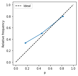

Let us wrap into a function

def calib_curve(true, pred, n_bins = 10):
    splits_arr = np.linspace(0, 1, n_bins + 1)
    splits = np.digitize(pred, splits_arr)
    p_group = {}
    labels_pos = {}
    for group in np.unique(splits):
        p_group[group] = pred[splits==group]
        labels_pos[group] = true[splits==group]
    p_group_mean = {k:np.mean(v) for k, v in p_group.items()}
    fracs = {k:np.sum(v)*1.0/len(v) for k, v in labels_pos.items()}
    counts = np.array([len(v) for v in labels_pos.values()])
    return  np.array(list(p_group_mean.values())), np.array(list(fracs.values())), counts

from sklearn.calibration import calibration_curve, CalibrationDisplay

prob_true, prob_pred = calibration_curve(true_labels, p, n_bins=3)

prob_true

array([0.33333333, 0.5       , 0.8       ])

prob_pred

array([0.16666667, 0.45      , 0.82      ])

p_ours, p_hat_ours, count = calib_curve(true_labels, p, 3)
p_ours

array([0.16666667, 0.45      , 0.82      ])

Expected Calibration Error

(np.abs(p_ours-p_hat_ours)*count).mean()

0.23333333333333336

from sklearn.datasets import make_classification

X, y = make_classification(n_features=2, n_informative=2, n_redundant=0, random_state=0)

plt.scatter(X[:, 0], X[:, 1], c = y)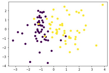

from sklearn.linear_model import LogisticRegression

lr = LogisticRegression()

lr.fit(X, y)

LogisticRegression()

In a Jupyter environment, please rerun this cell to show the HTML representation or trust the notebook.
On GitHub, the HTML representation is unable to render, please try loading this page with nbviewer.org.

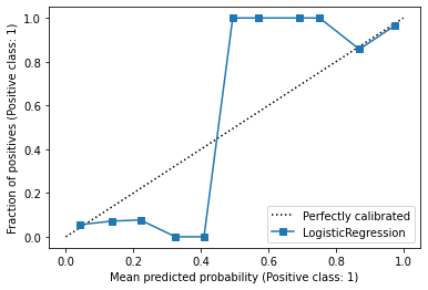
display = CalibrationDisplay.from_estimator(
        lr,
        X,
        y,
        n_bins=11,
)

pred_p = lr.predict_proba(X)[:, 1]

probs, fractions, counts  = calib_curve(y, pred_p, 11)

plt.plot(probs, fractions, marker='^')
plt.xlabel("p")
plt.ylabel("Relative frequency")

plt.plot([0, 1], [0, 1], color='k', ls='--', label='Ideal')
plt.legend()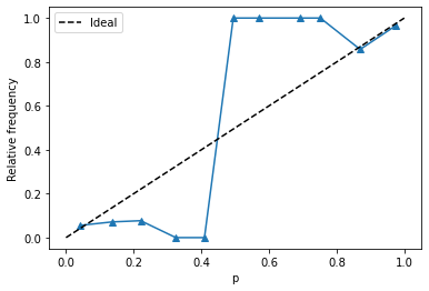

plt.hist(pred_p);

(np.abs(probs-fractions)*counts).mean()

0.9530316314463302

counts

array([18, 14, 13,  4,  2,  4,  2,  2,  6,  7, 28])