Temperature Scaling in Softmax: Controlling Randomness in Language Models

Exploring how temperature scaling affects the randomness and diversity of language model outputs through mathematical analysis and interactive visualizations
deep learning
natural language processing
softmax
temperature scaling
text generation
Author

Nipun Batra

Published

July 9, 2025

Temperature Scaling in Softmax: The Mathematics

Temperature scaling modifies the softmax function to control the “sharpness” of the probability distribution. The standard softmax function is:

\[\text{softmax}(x_i) = \frac{e^{x_i}}{\sum_{j=1}^{n} e^{x_j}}\]

With temperature scaling, we introduce a temperature parameter \(T\):

\[\text{softmax}_T(x_i) = \frac{e^{x_i/T}}{\sum_{j=1}^{n} e^{x_j/T}}\]

Effects of Temperature:

  • T = 1: Standard softmax (no scaling)
  • T > 1: Higher temperature → More uniform distribution → More randomness
  • T < 1: Lower temperature → Sharper distribution → More deterministic
  • T → 0: Distribution becomes one-hot (argmax)
  • T → ∞: Distribution becomes uniform

Entropy and Diversity:

The entropy of a probability distribution measures its randomness: \[H(p) = -\sum_{i=1}^{n} p_i \log p_i\]

Higher temperature typically leads to higher entropy and more diverse outputs.

Imports and Setup

Let’s import the necessary libraries and set up our environment:

from transformers import AutoModelForCausalLM, AutoTokenizer
import torch
import numpy as np
import matplotlib.pyplot as plt
import pandas as pd
from collections import Counter
from scipy.stats import entropy

# Rich imports for better formatting
from rich.console import Console
from rich.table import Table
from rich.text import Text
from rich import print as rprint

# Initialize rich console
console = Console()

All necessary libraries loaded for language modeling, visualization, and rich formatting.

Visual Demonstration

Let’s create a visual diagram showing how temperature affects probability distributions:

# Set up prettier matplotlib styling
plt.rcParams.update({
    'font.size': 12,
    'axes.labelsize': 14,
    'axes.titlesize': 16,
    'xtick.labelsize': 12,
    'ytick.labelsize': 12,
    'legend.fontsize': 12,
    'figure.titlesize': 18
})

# Create sample logits and temperature ranges
logits = np.array([2.0, 1.0, 0.5, 0.2, 0.1])
temperatures = [0.1, 0.5, 1.0, 2.0, 5.0]

# Create subplots with better styling
fig, axes = plt.subplots(1, len(temperatures), figsize=(20, 5))
colors = ['#FF6B6B', '#4ECDC4', '#45B7D1', '#96CEB4', '#FECA57']

for i, temp in enumerate(temperatures):
    # Calculate probabilities for this temperature
    scaled_logits = logits / temp
    probs = np.exp(scaled_logits) / np.sum(np.exp(scaled_logits))
    
    # Create DataFrame for this temperature
    df_temp = pd.DataFrame({
        'Token': [f'Token_{j}' for j in range(len(logits))],
        'Probability': probs
    })
    
    # Plot distribution with better styling
    bars = axes[i].bar(df_temp['Token'], df_temp['Probability'], 
                      color=colors[i], alpha=0.8, edgecolor='white', linewidth=1.5)
    
    # Bold T=1.0
    title_weight = 'bold' if temp == 1.0 else 'normal'
    title_size = 16 if temp == 1.0 else 14
    axes[i].set_title(f'Temperature = {temp}', fontweight=title_weight, fontsize=title_size)
    
    axes[i].set_ylabel('Probability', fontweight='bold')
    axes[i].set_ylim(0, 1.1)
    axes[i].tick_params(axis='x', rotation=45)
    axes[i].grid(True, alpha=0.3, linestyle='--')
    axes[i].set_facecolor('#F8F9FA')
    
    # Add probability values on top of bars
    for bar, prob in zip(bars, probs):
        axes[i].text(bar.get_x() + bar.get_width()/2., bar.get_height() + 0.02,
                    f'{prob:.2f}', ha='center', va='bottom', fontweight='bold', fontsize=10)

plt.suptitle('Temperature Scaling Effects: Distribution Shape Changes', 
            fontsize=20, fontweight='bold', y=1.02)
plt.tight_layout()
plt.show()

This diagram clearly shows how temperature reshapes probability distributions - low temperatures create peaked distributions while high temperatures flatten them.

Model Setup

Load a language model to explore temperature effects in practice:

model_name = "distilgpt2"
tokenizer = AutoTokenizer.from_pretrained(model_name)
model = AutoModelForCausalLM.from_pretrained(model_name)

# Set padding token to avoid warnings
tokenizer.pad_token = tokenizer.eos_token

DistilGPT2 loaded with proper tokenizer configuration.

Example Prompt

Let’s start with a simple prompt to analyze:

prompt = "In the future, AI will"
input_ids = tokenizer(prompt, return_tensors="pt").input_ids
print("Input IDs:", input_ids)
print("Vocabulary size:", model.config.vocab_size)
Input IDs: tensor([[ 818,  262, 2003,   11, 9552,  481]])
Vocabulary size: 50257

The model converts text to token IDs and works with a vocabulary of 50,257 tokens.

Text Generation with Low Temperature

Generate text with very low temperature to see deterministic behavior:

output = model.generate(
    input_ids,
    do_sample=True,
    temperature=0.01,
    max_new_tokens=20,
    top_k=50,
    pad_token_id=tokenizer.eos_token_id,
    attention_mask=torch.ones_like(input_ids)
)

decoded = tokenizer.decode(output[0], skip_special_tokens=True)
print("Generated text:", decoded)
Generated text: In the future, AI will be able to do things like make people smarter, more intelligent, more intelligent, more intelligent, more

Low temperature produces repetitive, deterministic text.

Logits Analysis

Let’s examine the raw logits and probabilities for next token prediction:

# Get the logits for prediction
with torch.no_grad():
    outputs = model(input_ids)
    logits = outputs.logits
    # Show logits and probabilities for top 10 tokens
    top_logits, top_indices = torch.topk(logits[0, -1], k=10)
    top_probs = torch.softmax(top_logits, dim=0)
    top_tokens = [tokenizer.decode([idx]) for idx in top_indices]
    
    # Create a clean table
    table = Table(title="Top 10 Token Predictions")
    table.add_column("Rank", style="dim")
    table.add_column("Token", style="cyan")
    table.add_column("Logit", style="magenta")
    table.add_column("Probability", style="green")
    
    for i, (token, logit, prob) in enumerate(zip(top_tokens, top_logits, top_probs)):
        table.add_row(
            str(i + 1),
            repr(token),
            f"{logit.item():.4f}",
            f"{prob.item():.4f}"
        )
    
    console.print(table)
           Top 10 Token Predictions            
┏━━━━━━┳━━━━━━━━━━━━━┳━━━━━━━━━━┳━━━━━━━━━━━━━┓
┃ Rank  Token        Logit     Probability ┃
┡━━━━━━╇━━━━━━━━━━━━━╇━━━━━━━━━━╇━━━━━━━━━━━━━┩
│ 1     ' be'        -63.5934  0.5269      │
│ 2     ' have'      -64.7306  0.1690      │
│ 3     ' need'      -65.5254  0.0763      │
│ 4     ' become'    -65.8555  0.0549      │
│ 5     ' not'       -66.0847  0.0436      │
│ 6     ' also'      -66.4207  0.0312      │
│ 7     ' take'      -66.5617  0.0271      │
│ 8     ' continue'  -66.5808  0.0266      │
│ 9     ' make'      -66.6369  0.0251      │
│ 10    ' only'      -66.8984  0.0193      │
└──────┴─────────────┴──────────┴─────────────┘

The model shows clear preference for certain tokens, with “be” having the highest probability.

Token Sampling

Sample tokens from the probability distribution to see randomness in action:

# Sample tokens from the distribution
sampled_indices = torch.multinomial(top_probs, num_samples=100, replacement=True)
sampled_tokens = [top_tokens[idx] for idx in sampled_indices]

# Display sample using Rich
rprint("Sample of tokens:")
rprint(" ".join([f"[cyan]{token}[/cyan]" for token in sampled_tokens[:20]]))

# Count occurrences and display in Rich table
token_counts = Counter(sampled_tokens)

# Create Rich table for token counts
table = Table(title="Token Counts from 100 Samples")
table.add_column("Token", style="cyan")
table.add_column("Count", style="green")
table.add_column("Percentage", style="yellow")

for token, count in token_counts.most_common():
    percentage = (count / 100) * 100
    table.add_row(token, str(count), f"{percentage:.1f}%")

console.print(table)
Sample of tokens:
 be  make  make  be  not  have  become  be  have  have  have  be  be  need  become  need  also  be  also  be
  Token Counts from 100 Samples   
┏━━━━━━━━━━━┳━━━━━━━┳━━━━━━━━━━━━┓
┃ Token      Count  Percentage ┃
┡━━━━━━━━━━━╇━━━━━━━╇━━━━━━━━━━━━┩
│  be        53     53.0%      │
│  have      16     16.0%      │
│  become    9      9.0%       │
│  need      9      9.0%       │
│  also      4      4.0%       │
│  make      3      3.0%       │
│  not       2      2.0%       │
│  take      2      2.0%       │
│  continue  2      2.0%       │
└───────────┴───────┴────────────┘

Token counts from 100 samples reflect the underlying probability distribution.

Temperature Scaling Comparison

Compare extreme temperature values to see dramatic differences:

# Temperature scaling comparison across multiple temperatures
temperature_values = [0.01, 0.1, 0.5, 1.0, 2.0, 5.0, 100.0]

# Calculate probabilities for each temperature
temp_results = {}
for temp in temperature_values:
    scaled_logits = logits / temp
    top_logits_temp, top_indices_temp = torch.topk(scaled_logits[0, -1], k=10)
    top_probs_temp = torch.softmax(top_logits_temp, dim=0)
    temp_results[temp] = {
        'probs': top_probs_temp,
        'tokens': [tokenizer.decode([idx]) for idx in top_indices_temp]
    }

# Create comprehensive comparison table
table = Table(title="Temperature Scaling: Full Spectrum Comparison")
table.add_column("Rank", style="dim")
table.add_column("Token", style="cyan")

for temp in temperature_values:
    if temp == 1.0:
        table.add_column(f"**T={temp}**", style="bold green")  # Bold T=1
    else:
        table.add_column(f"T={temp}", style="green" if temp > 1.0 else "red")

for i in range(10):
    row_data = [str(i + 1), repr(temp_results[temperature_values[0]]['tokens'][i])]
    
    for temp in temperature_values:
        prob = temp_results[temp]['probs'][i].item()
        row_data.append(f"{prob:.4f}")
    
    table.add_row(*row_data)

console.print(table)
                      Temperature Scaling: Full Spectrum Comparison                      
┏━━━━━━┳━━━━━━━━━━━━━┳━━━━━━━━┳━━━━━━━━┳━━━━━━━━┳━━━━━━━━━━━┳━━━━━━━━┳━━━━━━━━┳━━━━━━━━━┓
┃ Rank  Token        T=0.01  T=0.1   T=0.5   **T=1.0**  T=2.0   T=5.0   T=100.0 ┃
┡━━━━━━╇━━━━━━━━━━━━━╇━━━━━━━━╇━━━━━━━━╇━━━━━━━━╇━━━━━━━━━━━╇━━━━━━━━╇━━━━━━━━╇━━━━━━━━━┩
│ 1     ' be'        1.0000  1.0000  0.8667  0.5269     0.2731  0.1550  0.1023  │
│ 2     ' have'      0.0000  0.0000  0.0891  0.1690     0.1547  0.1235  0.1012  │
│ 3     ' need'      0.0000  0.0000  0.0182  0.0763     0.1039  0.1053  0.1004  │
│ 4     ' become'    0.0000  0.0000  0.0094  0.0549     0.0881  0.0986  0.1000  │
│ 5     ' not'       0.0000  0.0000  0.0059  0.0436     0.0786  0.0942  0.0998  │
│ 6     ' also'      0.0000  0.0000  0.0030  0.0312     0.0664  0.0881  0.0995  │
│ 7     ' take'      0.0000  0.0000  0.0023  0.0271     0.0619  0.0856  0.0993  │
│ 8     ' continue'  0.0000  0.0000  0.0022  0.0266     0.0613  0.0853  0.0993  │
│ 9     ' make'      0.0000  0.0000  0.0020  0.0251     0.0596  0.0843  0.0992  │
│ 10    ' only'      0.0000  0.0000  0.0012  0.0193     0.0523  0.0800  0.0990  │
└──────┴─────────────┴────────┴────────┴────────┴───────────┴────────┴────────┴─────────┘

High temperature creates uniform distribution while low temperature creates deterministic selection.

Temperature Analysis

Analyze how different temperatures affect probability distributions and entropy:

# Function to analyze temperature effects
def analyze_temperature_effects(logits, temperatures, top_k=10):
    results = []
    for temp in temperatures:
        scaled_logits = logits / temp
        probs = torch.softmax(scaled_logits, dim=-1)
        
        # Get top-k tokens
        top_probs, top_indices = torch.topk(probs[0, -1], k=top_k)
        top_tokens = [tokenizer.decode([idx]) for idx in top_indices]
        
        # Calculate entropy
        prob_dist = probs[0, -1].cpu().numpy()
        entropy_value = entropy(prob_dist)
        
        for i, (token, prob) in enumerate(zip(top_tokens, top_probs)):
            results.append({
                'temperature': temp,
                'token': token,
                'probability': prob.item(),
                'rank': i + 1,
                'entropy': entropy_value
            })
    
    return results

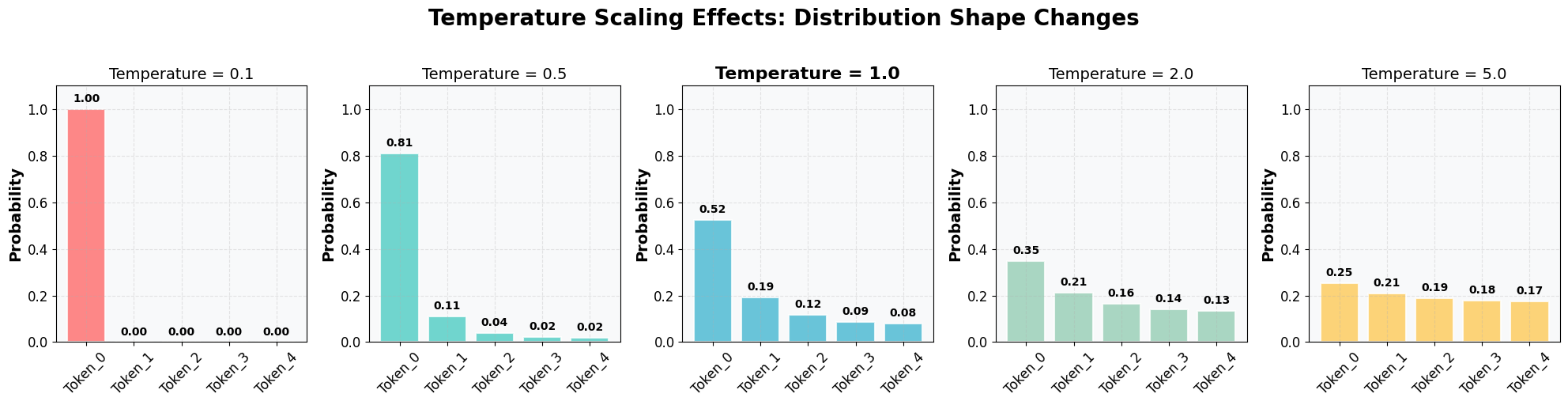
# Test with different temperature values
temperatures = [0.1, 0.5, 1.0, 2.0, 5.0]
results = analyze_temperature_effects(logits, temperatures)

# Create prettier visualizations
plt.rcParams.update({
    'font.size': 12,
    'axes.labelsize': 14,
    'axes.titlesize': 16,
    'xtick.labelsize': 12,
    'ytick.labelsize': 12,
    'legend.fontsize': 12,
    'figure.titlesize': 18
})

fig, axes = plt.subplots(1, 2, figsize=(16, 6))

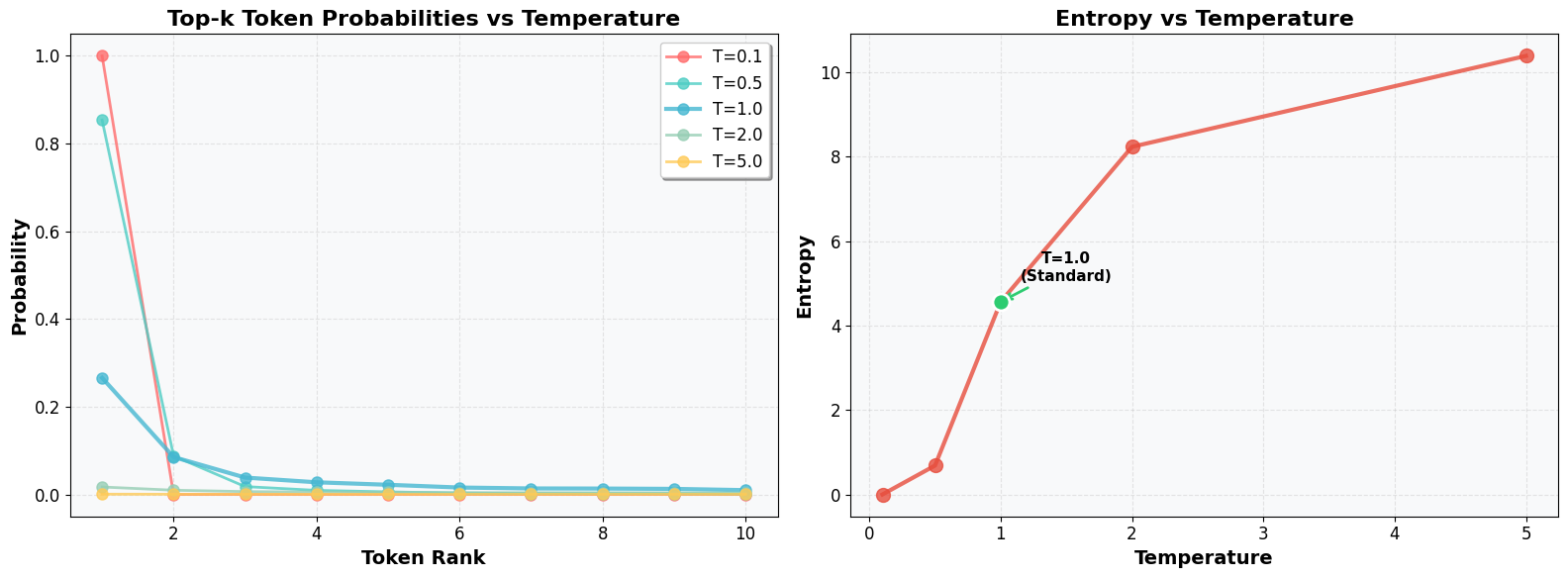
# Plot 1: Top-k probabilities with better styling
colors = ['#FF6B6B', '#4ECDC4', '#45B7D1', '#96CEB4', '#FECA57']
for i, temp in enumerate(temperatures):
    temp_data = [r for r in results if r['temperature'] == temp]
    ranks = [r['rank'] for r in temp_data]
    probs = [r['probability'] for r in temp_data]
    
    linewidth = 3 if temp == 1.0 else 2
    axes[0].plot(ranks, probs, 'o-', label=f'T={temp}', 
                color=colors[i], linewidth=linewidth, markersize=8, alpha=0.8)

axes[0].set_xlabel('Token Rank', fontweight='bold')
axes[0].set_ylabel('Probability', fontweight='bold')
axes[0].set_title('Top-k Token Probabilities vs Temperature', fontweight='bold')
axes[0].legend(frameon=True, fancybox=True, shadow=True)
axes[0].grid(True, alpha=0.3, linestyle='--')
axes[0].set_facecolor('#F8F9FA')

# Plot 2: Entropy vs Temperature with better styling
entropies = []
for temp in temperatures:
    temp_entropy = [r['entropy'] for r in results if r['temperature'] == temp][0]
    entropies.append(temp_entropy)

axes[1].plot(temperatures, entropies, 'o-', color='#E74C3C', 
            linewidth=3, markersize=10, alpha=0.8)
axes[1].set_xlabel('Temperature', fontweight='bold')
axes[1].set_ylabel('Entropy', fontweight='bold')
axes[1].set_title('Entropy vs Temperature', fontweight='bold')
axes[1].grid(True, alpha=0.3, linestyle='--')
axes[1].set_facecolor('#F8F9FA')

# Highlight T=1.0 on entropy plot
idx_1 = temperatures.index(1.0)
axes[1].scatter(1.0, entropies[idx_1], color='#2ECC71', s=150, 
               zorder=5, edgecolors='white', linewidth=2)
axes[1].annotate('T=1.0\n(Standard)', xy=(1.0, entropies[idx_1]), 
                xytext=(1.5, entropies[idx_1] + 0.5),
                arrowprops=dict(arrowstyle='->', color='#2ECC71', lw=2),
                fontsize=11, ha='center', fontweight='bold')

plt.tight_layout()
plt.show()

Higher temperatures lead to flatter distributions and higher entropy, confirming the mathematical relationship.

Diverse Examples Across Domains

Test temperature effects on different types of content:

def generate_comparison_examples():
    """Generate examples across different domains to show temperature effects"""
    
    examples = [
        ("The scientific method involves", "Science"),
        ("To solve the equation x^2 - 4x + 3 = 0,", "Mathematics"),
        ("In Shakespeare's time, the theater", "Literature/English")
    ]
    
    temperatures = [0.3, 1.0, 2.0]
    
    for prompt, domain in examples:
        rprint(f"\n[bold]{domain.upper()}[/bold]")
        rprint(f"Prompt: '{prompt}'")
        rprint("-" * 50)
        
        input_ids = tokenizer(prompt, return_tensors="pt").input_ids
        
        for temp in temperatures:
            rprint(f"\n[cyan]Temperature {temp}:[/cyan]")
            for i in range(3):  # Generate 3 samples per temperature
                output = model.generate(
                    input_ids,
                    do_sample=True,
                    temperature=temp,
                    max_new_tokens=15,
                    top_k=50,
                    pad_token_id=tokenizer.eos_token_id,
                    attention_mask=torch.ones_like(input_ids)
                )
                
                generated_text = tokenizer.decode(output[0], skip_special_tokens=True)
                new_text = generated_text[len(prompt):].strip()
                rprint(f"  Sample {i+1}: {new_text}")
        
        print()

generate_comparison_examples()
SCIENCE
Prompt: 'The scientific method involves'
--------------------------------------------------
Temperature 0.3:
  Sample 1: the use of a single, single, single, single-digit number.
  Sample 2: a series of steps to achieve a specific goal. For example, the goal
  Sample 3: taking a single molecule of a molecule of a molecule of a molecule of a
Temperature 1.0:
  Sample 1: two elements: a measurement of the quality of the water and a measurement of
  Sample 2: measuring the concentration of a large number of nucleic acids. (See a
  Sample 3: measuring all sorts of atoms using two different atomic weights, called the ‴
Temperature 2.0:
  Sample 1: some complicated equations such that the equations simply must exist before applying force. In
  Sample 2: determining each set of biological pathways to change each phenotype based on that pathway.
  Sample 3: using samples in real and made use of pure glass; with a special lens
MATHEMATICS
Prompt: 'To solve the equation x^2 - 4x + 3 = 0,'
--------------------------------------------------
Temperature 0.3:
  Sample 1: 2x + 3 = 0, 2x + 3 = 0, 2
  Sample 2: and then it is the same as x^2 + 4x + 4
  Sample 3: x^2 - 4x + 3 = 0, x^2 -
Temperature 1.0:
  Sample 1: 3x = 1, 4x = 2, 4x = 3,
  Sample 2: 0 , and 1 )


The idea is simple.
  Sample 3: but the answer at 1x is the same as with m^2 -
Temperature 2.0:
  Sample 1: where * x=A.add(-10, 0 / B)
  Sample 2: ‰
  Sample 3: 4 ( \times f(-x)). Note the error of z(5
LITERATURE/ENGLISH
Prompt: 'In Shakespeare's time, the theater'
--------------------------------------------------
Temperature 0.3:
  Sample 1: was a kind of theater, a kind of theater, a kind of theater
  Sample 2: was a place where people could play Shakespeare and Shakespeare. The theater was a
  Sample 3: was a kind of theater where the audience could see the characters and the characters
Temperature 1.0:
  Sample 1: is a work of art and creativity.


He and his wife
  Sample 2: and the music are also known for using Shakespeare's "soul with him
  Sample 3: 's most famous poet, Thomas Edison, drew its light on his favorite verse
Temperature 2.0:
  Sample 1: troupe was founded by British writer Stephen King at around that stage. Here
  Sample 2: might have had better management because of the lack of quality of production at a
  Sample 3: director himself had, as Sir Francis Molloy had hinted about a �

Multiple samples reveal consistency patterns at low temperatures and diversity at high temperatures across all domains.

Practical Applications

Use Cases

  • Low Temperature (0.1-0.5): Code generation, technical docs, factual content
  • Medium Temperature (0.7-1.2): Creative writing, chatbots, general text
  • High Temperature (1.5-3.0): Brainstorming, fiction, diverse idea generation

Quick Guidelines

  • Start with T=1.0 as baseline
  • Lower temperature for consistency and accuracy
  • Higher temperature for creativity and diversity

Conclusion

Temperature scaling is a simple yet powerful technique for controlling language model randomness:

  • T < 1: More deterministic, consistent outputs
  • T = 1: Standard softmax behavior
  • T > 1: More random, diverse outputs

Monitor entropy to quantify diversity. Temperature remains one of the most practical tools for controlling LLM behavior.

References

Code and Implementation

  • Temperature Scaling Repository: https://github.com/gpleiss/temperature_scaling
  • Twitter Discussion: https://x.com/akshay_pachaar/status/1942201076767412307

Academic Sources

  • Hinton, G. et al. (2015): “Distilling the Knowledge in a Neural Network” - Original paper introducing temperature in knowledge distillation
  • Guo, C. et al. (2017): “On Calibration of Modern Neural Networks” - ICML paper on temperature scaling for calibration
  • Goodfellow, I. et al. (2016): “Deep Learning” - Chapter 6 covers softmax and temperature scaling
  • Bishop, C. (2006): “Pattern Recognition and Machine Learning” - Chapter 4 discusses softmax temperature

Textbooks

  • “Deep Learning” by Goodfellow, Bengio, and Courville - Comprehensive coverage of softmax and sampling techniques
  • “Pattern Recognition and Machine Learning” by Christopher Bishop - Mathematical foundations of probability distributions
  • “The Elements of Statistical Learning” by Hastie, Tibshirani, and Friedman - Statistical perspective on temperature scaling