Learning HMM parameters from data: continuous (Gaussian) emissions
The previous post learned a discrete HMM – the observation was a category (walk/shop/clean). But most signals we actually measure are real numbers: temperature, acceleration, and – the case we are building toward – the power drawn by an appliance.
So we swap the categorical emission for a Gaussian one: each hidden state has a mean level \(\mu_k\) and a noise spread \(\sigma_k\), and the observation is \(y_t \sim \mathcal{N}(\mu_{z_t}, \sigma_{z_t})\). This is the entire change to the model – everything else (priors, enumeration, SVI) is exactly as before. Varying the emission is varying the graphical model, and the inference machinery just follows along.
As before: fix true parameters, generate data, learn them back, check.
Code
import torchimport pyroimport pyro.distributions as distfrom pyro.ops.indexing import Vindexfrom pyro.infer import SVI, TraceEnum_ELBO, config_enumerate, infer_discretefrom pyro.infer.autoguide import AutoDelta, init_to_samplefrom pyro import poutineimport numpy as npimport pandas as pdimport matplotlib.pyplot as plt%matplotlib inline%config InlineBackend.figure_format ='retina'pyro.set_rng_seed(0)plt.rcParams.update({"figure.dpi": 110, "font.size": 11})
/Users/nipun/git/hmm/.venv/lib/python3.13/site-packages/tqdm/auto.py:21: TqdmWarning: IProgress not found. Please update jupyter and ipywidgets. See https://ipywidgets.readthedocs.io/en/stable/user_install.html
  from .autonotebook import tqdm as notebook_tqdm
A Gaussian-emission HMM
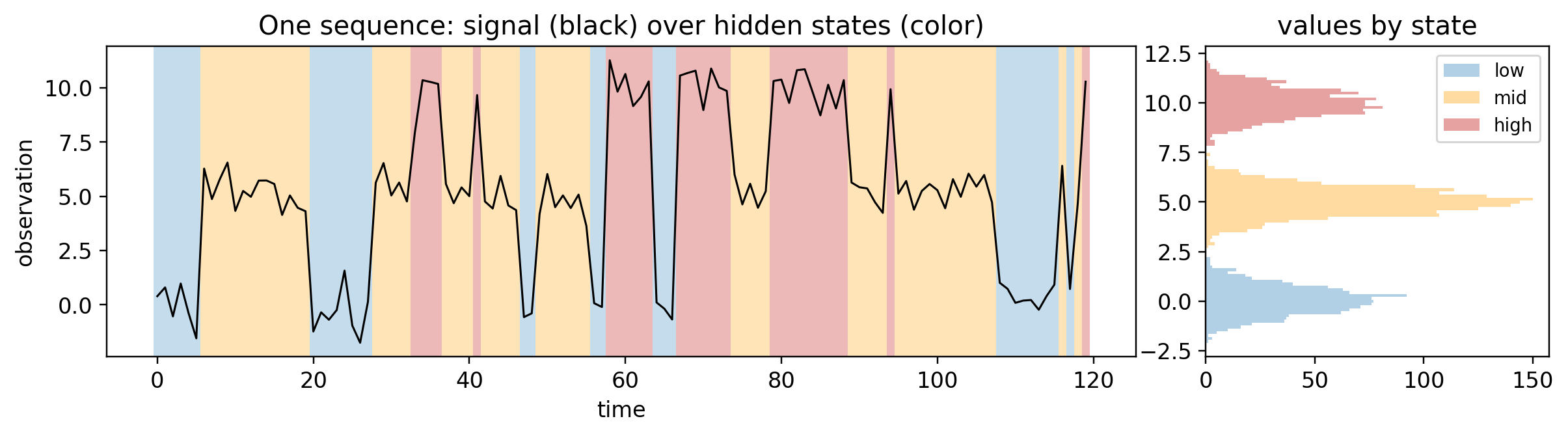
Think of a signal that hops between a few levels and stays in each for a while – a device idling, running, and boosting, say. We use three states with distinct mean levels and small noise. These are the true parameters we will hide from the learner.
Code
states = ["low", "mid", "high"]K =3pi_true = torch.tensor([0.5, 0.3, 0.2])A_true = torch.tensor([[0.80, 0.15, 0.05], [0.10, 0.80, 0.10], [0.05, 0.15, 0.80]])mu_true = torch.tensor([0.0, 5.0, 10.0]) # mean level per statesd_true = torch.tensor([0.7, 0.7, 0.7]) # noise per statedef generate(num_seqs, T, seed=1): g = torch.Generator().manual_seed(seed) obs = torch.zeros(num_seqs, T) Z = torch.zeros(num_seqs, T, dtype=torch.long)for s inrange(num_seqs): z = torch.multinomial(pi_true, 1, generator=g).item()for t inrange(T):if t >0: z = torch.multinomial(A_true[z], 1, generator=g).item() Z[s, t] = z obs[s, t] = mu_true[z] + sd_true[z] * torch.randn(1, generator=g).item()return obs, Zobs, Z = generate(num_seqs=30, T=120, seed=1)print("data:", tuple(obs.shape))
data: (30, 120)
Code
colors = ["#9ec5e0", "#ffd28a", "#e08a8a"]fig, (a1, a2) = plt.subplots(1, 2, figsize=(11, 3.2), gridspec_kw={"width_ratios": [3, 1]})seq = obs[0].numpy(); zs = Z[0].numpy(); T =len(seq)for t inrange(T): a1.axvspan(t-0.5, t+0.5, color=colors[zs[t]], alpha=0.6, lw=0)a1.plot(seq, color="k", lw=1)a1.set_title("One sequence: signal (black) over hidden states (color)")a1.set_xlabel("time"); a1.set_ylabel("observation")for k inrange(K): a2.hist(obs[Z == k].numpy(), bins=30, color=colors[k], alpha=0.8, label=states[k], orientation="horizontal")a2.set_title("values by state"); a2.legend(fontsize=9)plt.tight_layout(); plt.show()
The learnable model
Same skeleton as the discrete post. The hidden chain is unchanged; only the emission line differs – Normal instead of Categorical, with two sets of unknowns:
locs (the means \(\mu_k\)), given a broad Normal prior centred on the data;
scales (the spreads \(\sigma_k\)), given a positive LogNormal prior.
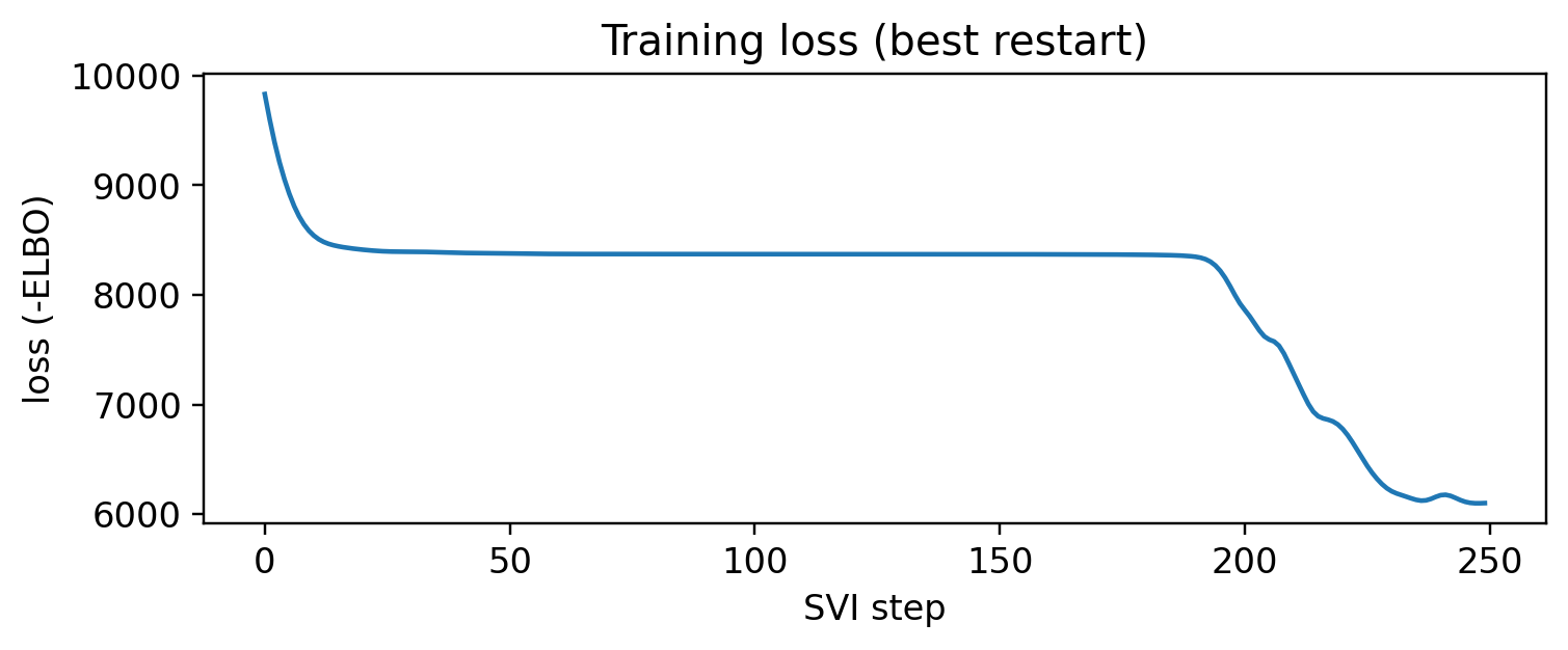
States are enumerated (summed out), parameters are point-estimated with AutoDelta, and we keep the best of a few random restarts since Gaussian EM is prone to local optima (e.g. two states grabbing one cluster).
Code
def model(obs, K): S, T = obs.shape probs_init = pyro.sample("probs_init", dist.Dirichlet(torch.ones(K))) probs_trans = pyro.sample("probs_trans", dist.Dirichlet(torch.ones(K, K)).to_event(1)) locs = pyro.sample("locs", dist.Normal(obs.mean(), 3* obs.std()).expand([K]).to_event(1)) scales = pyro.sample("scales", dist.LogNormal(0.0, 1.0).expand([K]).to_event(1))with pyro.plate("seqs", S, dim=-1): z =Nonefor t in pyro.markov(range(T)): probs = probs_init if t ==0else Vindex(probs_trans)[..., z, :] z = pyro.sample(f"z_{t}", dist.Categorical(probs), infer={"enumerate": "parallel"}) pyro.sample(f"y_{t}", dist.Normal(Vindex(locs)[..., z], Vindex(scales)[..., z]), obs=obs[:, t])def learn(obs, K, steps=300, lr=0.05, seed=0): pyro.clear_param_store(); pyro.set_rng_seed(seed) guide = AutoDelta(poutine.block(model, expose=["probs_init", "probs_trans", "locs", "scales"]), init_loc_fn=init_to_sample) svi = SVI(model, guide, pyro.optim.Adam({"lr": lr}), TraceEnum_ELBO(max_plate_nesting=1)) losses = [svi.step(obs, K) for _ inrange(steps)]return guide.median(obs, K), lossesdef learn_best(obs, K, steps=250, restarts=3): best =Nonefor r inrange(restarts): est, losses = learn(obs, K, steps=steps, seed=r)if best isNoneor losses[-1] < best[0]: best = (losses[-1], est, losses)return best[1], best[2]
Code
est, losses = learn_best(obs, K, steps=250, restarts=3)plt.figure(figsize=(7, 3))plt.plot(losses); plt.xlabel("SVI step"); plt.ylabel("loss (-ELBO)")plt.title("Training loss (best restart)"); plt.tight_layout(); plt.show()
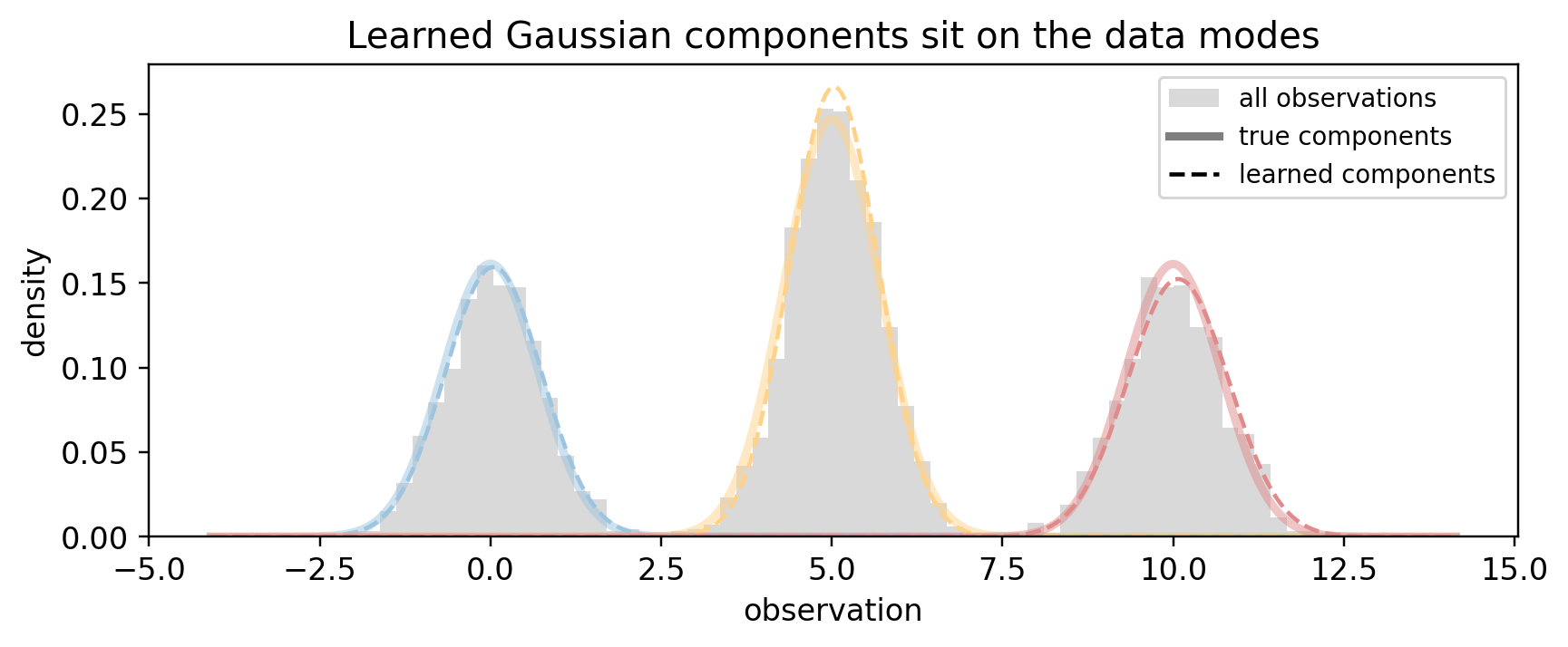
Recovered parameters
For continuous emissions, fixing label switching is easy: just sort the states by their learned mean. Then we compare to the (already sorted) ground truth.
/tmp/claude-501/ipykernel_63757/3648185236.py:6: DeprecationWarning: __array_wrap__ must accept context and return_scalar arguments (positionally) in the future. (Deprecated NumPy 2.0)
  true_pdf = occ[k].item() * np.exp(-0.5*((xs-mu_true[k].item())/sd_true[k].item())**2) / (sd_true[k].item()*np.sqrt(2*np.pi))
/tmp/claude-501/ipykernel_63757/3648185236.py:7: DeprecationWarning: __array_wrap__ must accept context and return_scalar arguments (positionally) in the future. (Deprecated NumPy 2.0)
  lrn_pdf  = occ[k].item() * np.exp(-0.5*((xs-mu_e[k].item())/sd_e[k].item())**2)       / (sd_e[k].item()*np.sqrt(2*np.pi))
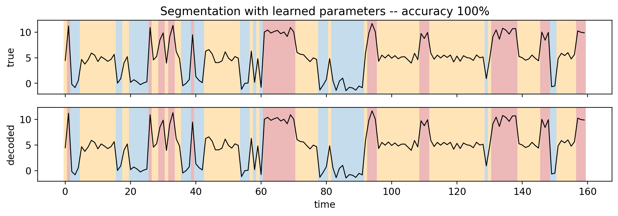
Decoding: segmenting a new signal
Finally, decode a fresh sequence with the learned parameters – i.e. label each time step with its most likely hidden state (Viterbi via infer_discrete) – and compare to the truth.
Code
def decode(pi, A, locs, scales, y):def m(y): z =Nonefor t in pyro.markov(range(len(y))): probs = pi if t ==0else Vindex(A)[..., z, :] z = pyro.sample(f"z_{t}", dist.Categorical(probs), infer={"enumerate": "parallel"}) pyro.sample(f"y_{t}", dist.Normal(Vindex(locs)[..., z], Vindex(scales)[..., z]), obs=y[t]) d = infer_discrete(config_enumerate(m, "parallel"), first_available_dim=-1, temperature=0) tr = poutine.trace(d).get_trace(y)return [int(tr.nodes[f"z_{t}"]["value"]) for t inrange(len(y))]y_test, z_test = generate(num_seqs=1, T=160, seed=77)y_test, z_test = y_test[0], z_test[0]# map learned-state indices back to sorted (true) labelsinv = torch.empty(K, dtype=torch.long); inv[order] = torch.arange(K)dec = [int(inv[d]) for d in decode(pi_e[inv], A_e[inv][:, inv], mu_e[inv], sd_e[inv], y_test)]acc =float(np.mean(np.array(dec) == z_test.numpy()))fig, (b1, b2) = plt.subplots(2, 1, figsize=(10, 3.6), sharex=True)for t inrange(len(y_test)): b1.axvspan(t-0.5, t+0.5, color=colors[int(z_test[t])], alpha=0.6, lw=0) b2.axvspan(t-0.5, t+0.5, color=colors[dec[t]], alpha=0.6, lw=0)b1.plot(y_test.numpy(), "k", lw=1); b2.plot(y_test.numpy(), "k", lw=1)b1.set_ylabel("true"); b2.set_ylabel("decoded"); b2.set_xlabel("time")b1.set_title(f"Segmentation with learned parameters -- accuracy {acc:.0%}")plt.tight_layout(); plt.show()
Wrap-up
A Gaussian-emission HMM was a one-line change from the discrete model, and Pyro recovered the means, spreads, and transitions almost exactly – then segmented an unseen signal at high accuracy.
This is precisely the model for a single appliance: its power trace hops between levels (off / on / boost), each a noisy mean. The catch in real homes is that we do not measure each appliance – we measure the sum at the meter. In the next post we put several of these Gaussian chains together into a factorial HMM, written with no Kronecker / product-state machinery, and disaggregate the total back into appliances in time linear in the number of appliances.