In this notebook, we will show how to compare different GP libraries to give the same loss for a simple GP regression problem.
Code
import numpy as npimport GPyimport gpytorchimport torchfrom jax.config import configimport jax.numpy as jnpimport optax as oximport jax.random as jrfrom jaxutils import Datasetimport jaxkern as jkimport gpjax as gpx# Enable Float64 for more stable matrix inversions.config.update("jax_enable_x64", True)key = jr.PRNGKey(123)from pprint import PrettyPrinterpp = PrettyPrinter(indent=4)# Generate the 1D regression datasetnp.random.seed(0)N =100X = np.linspace(0, 1, N).reshape(-1, 1)y = np.sin(2* np.pi * X).ravel() +0.05* np.random.randn(N)# Create the GPy modelkernel = GPy.kern.RBF(input_dim=1, lengthscale=1)gpy_model = GPy.models.GPRegression(X, y.reshape(-1, 1), kernel)# Evaluate the GPy lossgpy_loss =-gpy_model.log_likelihood()# Create the gpytorch modelclass GPRegressionModel(gpytorch.models.ExactGP):def__init__(self, train_x, train_y, likelihood):super(GPRegressionModel, self).__init__(train_x, train_y, likelihood)self.mean_module = gpytorch.means.ConstantMean()self.covar_module = gpytorch.kernels.ScaleKernel(gpytorch.kernels.RBFKernel())def forward(self, x): mean_x =self.mean_module(x) covar_x =self.covar_module(x)return gpytorch.distributions.MultivariateNormal(mean_x, covar_x)# Initialize the likelihood and modellikelihood_gpytorch = gpytorch.likelihoods.GaussianLikelihood()# Set likelihood noise to the GPy valuelikelihood_gpytorch.noise = gpy_model.likelihood.variance[0]gpytorch_model = GPRegressionModel(torch.from_numpy(X).float(), torch.from_numpy(y).float(), likelihood_gpytorch)# Set the kernel parameters to the GPy valuesgpytorch_model.covar_module.base_kernel.lengthscale = gpy_model.kern.lengthscale[0]gpytorch_model.covar_module.outputscale = gpy_model.kern.variance[0]# Confirm that the GPy and gpytorch models have the same parametersassert gpy_model.kern.lengthscale[0] == gpytorch_model.covar_module.base_kernel.lengthscale.item()assert gpy_model.kern.variance[0] == gpytorch_model.covar_module.outputscale.item()assert gpy_model.likelihood.variance[0] == gpytorch_model.likelihood.noise.item()# Find the gpytorch lossoutput = gpytorch_model(torch.from_numpy(X).float())# MLLmll = gpytorch.mlls.ExactMarginalLogLikelihood(likelihood_gpytorch, gpytorch_model)# Find the gpytorch lossgpytorch_loss =-mll(output, torch.from_numpy(y).float())# Print the lossesprint('GPy loss: {}'.format(gpy_loss))# We multiply by N because the gpytorch loss is the average loss per data pointprint('gpytorch loss: {}'.format(gpytorch_loss.item()*N))
# Set the GPy model parameters to the GPJax modelkernel = jk.RBF()prior = gpx.Prior(kernel=kernel)likelihood = gpx.Gaussian(num_datapoints=N)# Set the likelihood variance to the GPy modellikelihood.variance = gpy_model.likelihood.variance[0]
Code
parameter_state = gpx.initialise(prior, key)posterior = prior * likelihood# Set the kernel parameters to the GPy valuesparameter_state = gpx.initialise( posterior, key, kernel={"lengthscale": jnp.array([gpy_model.kern.lengthscale[0]]), "variance": jnp.array([gpy_model.kern.variance[0]])})
# Now train both the GPy, gpytorch and GPJax models and compare the losses and parameters# Use multiple restarts to find the best GPy model# Initialize the GPy model and then use the same hyperparameters in the gpytorch model# Use same optimizer and training iterations for both models# Train the GPy model with multiple restarts and 100 iterationsgpy_model.optimize(max_iters=100)# Train the gpytorch modelgpytorch_model.train()likelihood_gpytorch.train()# Train using Adamoptimizer = torch.optim.Adam(gpytorch_model.parameters(), lr=0.1) # Includes GaussianLikelihood parameters# "Loss" for GPs - the marginal log likelihoodmll = gpytorch.mlls.ExactMarginalLogLikelihood(likelihood_gpytorch, gpytorch_model)training_iter =100# Training loopfor i inrange(training_iter):# Zero backprop gradients optimizer.zero_grad()# Get output from model output = gpytorch_model(torch.from_numpy(X).float())# Calc loss and backprop gradients loss =-mll(output, torch.from_numpy(y).float()) loss.backward()print('Iter %d/%d - Loss: %.3f'% (i +1, training_iter, loss.item())) optimizer.step()# Print the GPy and gpytorch lossesprint('GPy loss: {}'.format(gpy_model.log_likelihood()))print('gpytorch loss: {}'.format(-mll(output, torch.from_numpy(y).float()).item()))
Iter 1/100 - Loss: 1.067
Iter 2/100 - Loss: 1.040
Iter 3/100 - Loss: 1.012
Iter 4/100 - Loss: 0.983
Iter 5/100 - Loss: 0.954
Iter 6/100 - Loss: 0.923
Iter 7/100 - Loss: 0.889
Iter 8/100 - Loss: 0.853
Iter 9/100 - Loss: 0.811
Iter 10/100 - Loss: 0.765
Iter 11/100 - Loss: 0.713
Iter 12/100 - Loss: 0.659
Iter 13/100 - Loss: 0.605
Iter 14/100 - Loss: 0.553
Iter 15/100 - Loss: 0.505
Iter 16/100 - Loss: 0.460
Iter 17/100 - Loss: 0.417
Iter 18/100 - Loss: 0.375
Iter 19/100 - Loss: 0.334
Iter 20/100 - Loss: 0.291
Iter 21/100 - Loss: 0.248
Iter 22/100 - Loss: 0.204
Iter 23/100 - Loss: 0.158
Iter 24/100 - Loss: 0.112
Iter 25/100 - Loss: 0.064
Iter 26/100 - Loss: 0.016
Iter 27/100 - Loss: -0.033
Iter 28/100 - Loss: -0.083
Iter 29/100 - Loss: -0.134
Iter 30/100 - Loss: -0.185
Iter 31/100 - Loss: -0.236
Iter 32/100 - Loss: -0.287
Iter 33/100 - Loss: -0.338
Iter 34/100 - Loss: -0.388
Iter 35/100 - Loss: -0.437
Iter 36/100 - Loss: -0.486
Iter 37/100 - Loss: -0.533
Iter 38/100 - Loss: -0.579
Iter 39/100 - Loss: -0.625
Iter 40/100 - Loss: -0.671
Iter 41/100 - Loss: -0.717
Iter 42/100 - Loss: -0.763
Iter 43/100 - Loss: -0.809
Iter 44/100 - Loss: -0.854
Iter 45/100 - Loss: -0.897
Iter 46/100 - Loss: -0.940
Iter 47/100 - Loss: -0.980
Iter 48/100 - Loss: -1.019
Iter 49/100 - Loss: -1.057
Iter 50/100 - Loss: -1.093
Iter 51/100 - Loss: -1.128
Iter 52/100 - Loss: -1.162
Iter 53/100 - Loss: -1.193
Iter 54/100 - Loss: -1.223
Iter 55/100 - Loss: -1.251
Iter 56/100 - Loss: -1.277
Iter 57/100 - Loss: -1.300
Iter 58/100 - Loss: -1.321
Iter 59/100 - Loss: -1.339
Iter 60/100 - Loss: -1.355
Iter 61/100 - Loss: -1.368
Iter 62/100 - Loss: -1.379
Iter 63/100 - Loss: -1.388
Iter 64/100 - Loss: -1.395
Iter 65/100 - Loss: -1.399
Iter 66/100 - Loss: -1.402
Iter 67/100 - Loss: -1.404
Iter 68/100 - Loss: -1.404
Iter 69/100 - Loss: -1.403
Iter 70/100 - Loss: -1.401
Iter 71/100 - Loss: -1.399
Iter 72/100 - Loss: -1.397
Iter 73/100 - Loss: -1.395
Iter 74/100 - Loss: -1.393
Iter 75/100 - Loss: -1.391
Iter 76/100 - Loss: -1.390
Iter 77/100 - Loss: -1.390
Iter 78/100 - Loss: -1.389
Iter 79/100 - Loss: -1.390
Iter 80/100 - Loss: -1.390
Iter 81/100 - Loss: -1.391
Iter 82/100 - Loss: -1.393
Iter 83/100 - Loss: -1.394
Iter 84/100 - Loss: -1.396
Iter 85/100 - Loss: -1.397
Iter 86/100 - Loss: -1.399
Iter 87/100 - Loss: -1.400
Iter 88/100 - Loss: -1.401
Iter 89/100 - Loss: -1.402
Iter 90/100 - Loss: -1.403
Iter 91/100 - Loss: -1.403
Iter 92/100 - Loss: -1.404
Iter 93/100 - Loss: -1.404
Iter 94/100 - Loss: -1.404
Iter 95/100 - Loss: -1.405
Iter 96/100 - Loss: -1.405
Iter 97/100 - Loss: -1.405
Iter 98/100 - Loss: -1.404
Iter 99/100 - Loss: -1.404
Iter 100/100 - Loss: -1.404
GPy loss: 140.45346660653308
gpytorch loss: -1.4040359258651733
Code
# Train the GPJax model# Use the same optimizer and training iterations as GPy and gpytorch# Create the GPJax modeloptimiser = ox.adam(learning_rate=0.01)inference_state = gpx.fit( objective=negative_mll, parameter_state=parameter_state, optax_optim=optimiser, num_iters=500,)
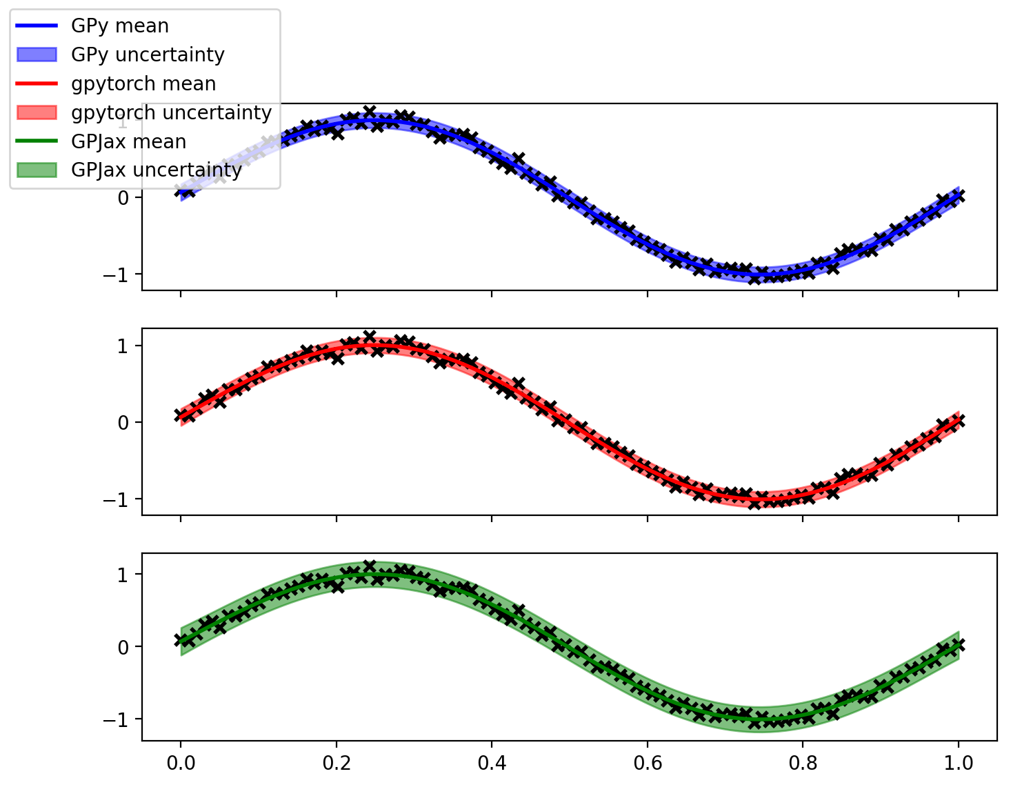
# plot the GPy, gpytorch and gpjax model predictions in 3 subplots sharing the x axis and having same ylimimport matplotlib.pyplot as plt%matplotlib inline# Retina display%config InlineBackend.figure_format ='retina'fig, axs = plt.subplots(3, 1, sharex=True, figsize=(8, 6))# Get the GPy predictionsgpy_mean, gpy_var = gpy_model.predict(X)# Get the gpytorch predictionsgpytorch_model.eval()likelihood_gpytorch.eval()with torch.no_grad(), gpytorch.settings.fast_pred_var(): observed_pred = likelihood_gpytorch(gpytorch_model(torch.from_numpy(X).float()))# Get the GPJax predictionslatent_dist = posterior(learned_params, ds)(X)predictive_dist = likelihood(learned_params, latent_dist)predictive_mean = predictive_dist.mean()predictive_std = predictive_dist.stddev()axs[0].plot(X, y, 'kx', mew=2)axs[0].plot(X, gpy_mean, 'b', lw=2, label='GPy mean')axs[1].plot(X, y, 'kx', mew=2)axs[1].plot(X, observed_pred.mean.numpy(), 'r', lw=2, label='gpytorch mean')axs[2].plot(X, y, 'kx', mew=2)axs[2].plot(X, predictive_mean, 'g', lw=2, label='GPJax mean')axs[0].fill_between(X.flatten(), gpy_mean.flatten() -2* np.sqrt(gpy_var.flatten()), gpy_mean.flatten() +2* np.sqrt(gpy_var.flatten()), alpha=0.5, color='blue', label='GPy uncertainty')# Get the lower and upper confidence bounds for the gpytorch modellower, upper = observed_pred.confidence_region()axs[1].fill_between(X.flatten(), lower.numpy().flatten(), upper.numpy().flatten(), alpha=0.5, color='red', label='gpytorch uncertainty')axs[2].fill_between(X.flatten(), predictive_mean.flatten() -2* predictive_std.flatten(), predictive_mean.flatten() +2* predictive_std.flatten(), alpha=0.5, color='green', label='GPJax uncertainty')fig.legend(loc='upper left')
/Users/nipun/miniconda3/lib/python3.9/site-packages/gpytorch/models/exact_gp.py:274: GPInputWarning:The input matches the stored training data. Did you forget to call model.train()?