Stacking (Ensemble Learning) – Nipun Batra Blog

In this post, we study a simple meta learning technique called Stacking

Code

import numpy as np
import pandas as pd
from sklearn.datasets import load_digits
from sklearn.model_selection import train_test_split
from sklearn.linear_model import LinearRegression
from sklearn.tree import DecisionTreeRegressor
import matplotlib.pyplot as plt

%config InlineBackend.figure_format = 'retina'

Create a noisy dataset using a 3rd degree polynomial

Code

np.random.seed(42)
x = np.linspace(-5, 5, 500)
f = lambda x: 0.1*x**3 + 0.2**x**2 + x + 4
y = f(x) + 0.05*np.random.normal(0, 100, 500)

plt.plot(x, y, 'o', label = 'data')
plt.plot(x, f(x), 'r', label = 'true')
plt.legend()

Create a train, validation and test set and plot them

Code

x_train, x_test, y_train, y_test = train_test_split(x, y, test_size=0.2)

x_train, x_val, y_train, y_val = train_test_split(x_train, y_train, test_size=0.2)

plt.plot(x_train, y_train, 'o', label = 'train', alpha = 0.5)
plt.plot(x_val, y_val, 'o', label = 'validation', alpha = 0.5)
plt.plot(x_test, y_test, 'o', label = 'test', alpha = 0.5)
plt.plot(x, f(x), 'r', label = 'true', lw=3)
plt.legend()

First layer of models

Code


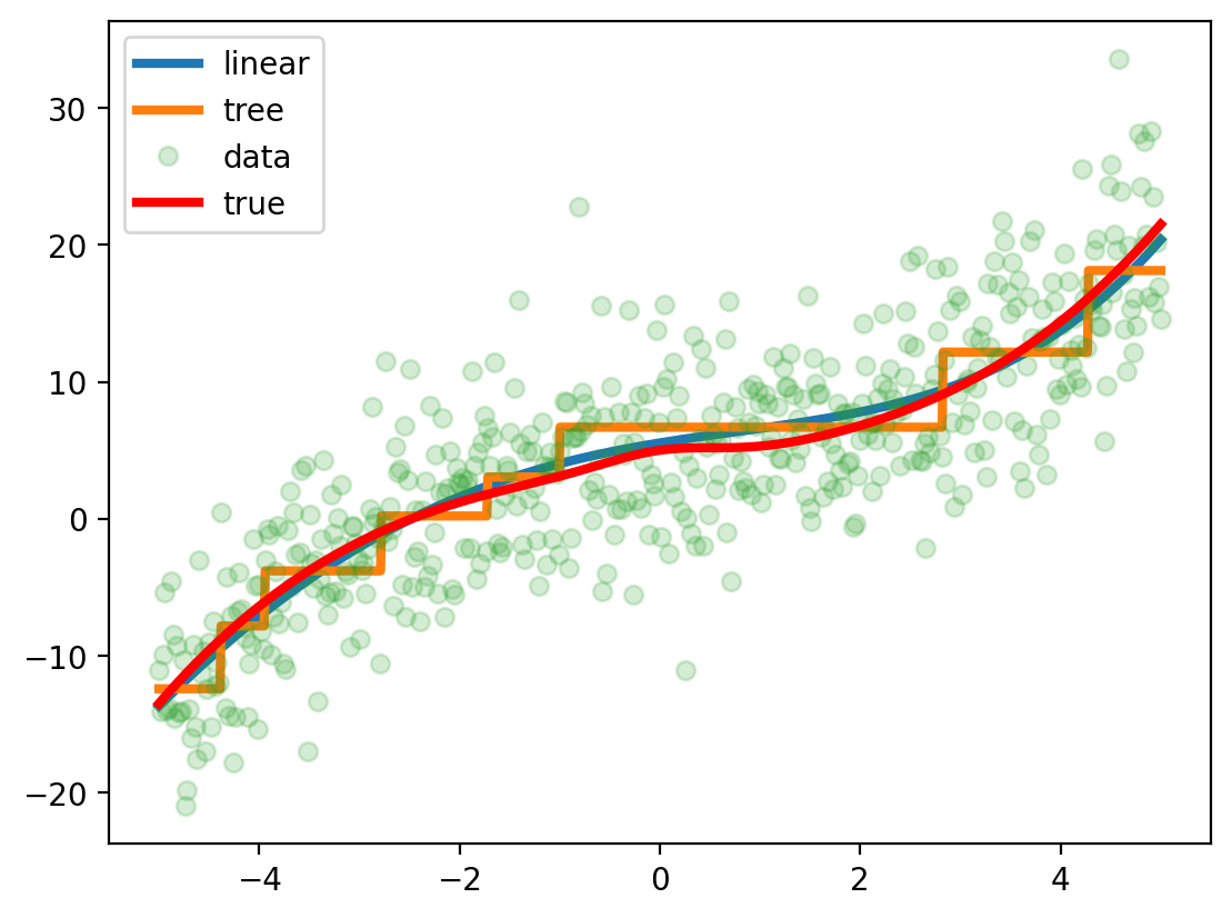
# Create a pipeline for linear regression using a polynomial feature transformer
from sklearn.pipeline import Pipeline
from sklearn.preprocessing import PolynomialFeatures

lr = Pipeline([('poly', PolynomialFeatures(degree=4)),
                ('linear', LinearRegression(fit_intercept=True))])

# Fit the model
lr.fit(x_train.reshape(-1, 1), y_train)


dt = DecisionTreeRegressor(max_depth=3)
_ = dt.fit(x_train.reshape(-1, 1), y_train)

Plot fits on 1d grid

Code

x_grid = np.linspace(-5, 5, 1000)
plt.plot(x_grid, lr.predict(x_grid.reshape(-1, 1)), label='linear', lw=3)
plt.plot(x_grid, dt.predict(x_grid.reshape(-1, 1)), label='tree', lw=3)
plt.plot(x, y, 'o', label='data', alpha=0.2)
plt.plot(x, f(x), 'r', label='true', lw=3)
plt.legend()

Code

# Train and test errors using sklearn.metrics.mean_squared_error
from sklearn.metrics import mean_squared_error

print('Train error linear: ', mean_squared_error(y_train, lr.predict(x_train.reshape(-1, 1))))
print('Test error linear: ', mean_squared_error(y_test, lr.predict(x_test.reshape(-1, 1))))
print('Train error tree: ', mean_squared_error(y_train, dt.predict(x_train.reshape(-1, 1))))
print('Test error tree: ', mean_squared_error(y_test, dt.predict(x_test.reshape(-1, 1))))

Train error linear:  23.00595790199621
Test error linear:  29.527934658588585
Train error tree:  21.577144246319136
Test error tree:  35.03378245179331

Second layer of models trained on the predictions of the first layer on the validation set

Code


# Create a new dataset with the predictions of the first layer
x_val_lr = lr.predict(x_val.reshape(-1, 1))
x_val_dt = dt.predict(x_val.reshape(-1, 1))
x_val_2d = np.column_stack((x_val_lr, x_val_dt))

# Fit a linear regression model on the new dataset
lr2 = LinearRegression()
lr2.fit(x_val_2d, y_val)

LinearRegression()

In a Jupyter environment, please rerun this cell to show the HTML representation or trust the notebook.
On GitHub, the HTML representation is unable to render, please try loading this page with nbviewer.org.

Code

# Errors on the test set

# Feature set for the test set
x_test_lr = lr.predict(x_test.reshape(-1, 1))
x_test_dt = dt.predict(x_test.reshape(-1, 1))
x_test_2d = np.column_stack((x_test_lr, x_test_dt))

# Test error
print('Test error META: ', mean_squared_error(y_test, lr2.predict(x_test_2d)))
print('Test error linear: ', mean_squared_error(y_test, lr.predict(x_test.reshape(-1, 1))))
print('Test error tree: ', mean_squared_error(y_test, dt.predict(x_test.reshape(-1, 1))))

Test error META:  29.023123374054247
Test error linear:  29.527934658588585
Test error tree:  35.03378245179331

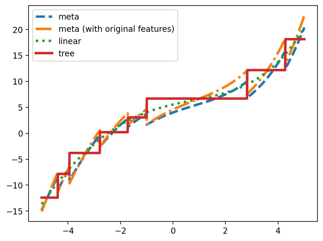
Include the raw features in the second layer

Code


# Feature set for the test set
x_test_3d = np.column_stack((x_test_lr, x_test_dt, x_test))

# Fit a linear regression model on the new dataset
lr3 = LinearRegression()
lr3.fit(x_test_3d, y_test)


# Test error
print('Test error Meta (with original features): ', mean_squared_error(y_test, lr3.predict(x_test_3d)))
print('Test error linear: ', mean_squared_error(y_test, lr.predict(x_test.reshape(-1, 1))))
print('Test error tree: ', mean_squared_error(y_test, dt.predict(x_test.reshape(-1, 1))))

Test error Meta (with original features):  27.931843644775036
Test error linear:  29.527934658588585
Test error tree:  35.03378245179331

Code

# Plot the fits on the 1d grid
x_grid_lr = lr.predict(x_grid.reshape(-1, 1))
x_grid_dt = dt.predict(x_grid.reshape(-1, 1))
x_grid_2d = np.column_stack((x_grid_lr, x_grid_dt))
x_grid_3d = np.column_stack((x_grid_lr, x_grid_dt, x_grid))

plt.plot(x_grid, lr2.predict(x_grid_2d), label='meta', lw=3, linestyle='--')
plt.plot(x_grid, lr3.predict(x_grid_3d), label='meta (with original features)', lw=3, linestyle='-.')
plt.plot(x_grid, lr.predict(x_grid.reshape(-1, 1)), label='linear', lw=3, ls=':')
plt.plot(x_grid, dt.predict(x_grid.reshape(-1, 1)), label='tree', lw=3, ls='-')
#plt.plot(x, y, 'o', label='data', alpha=0.2)
#plt.plot(x, f(x), 'r', label='true', lw=3)
plt.legend()

Code

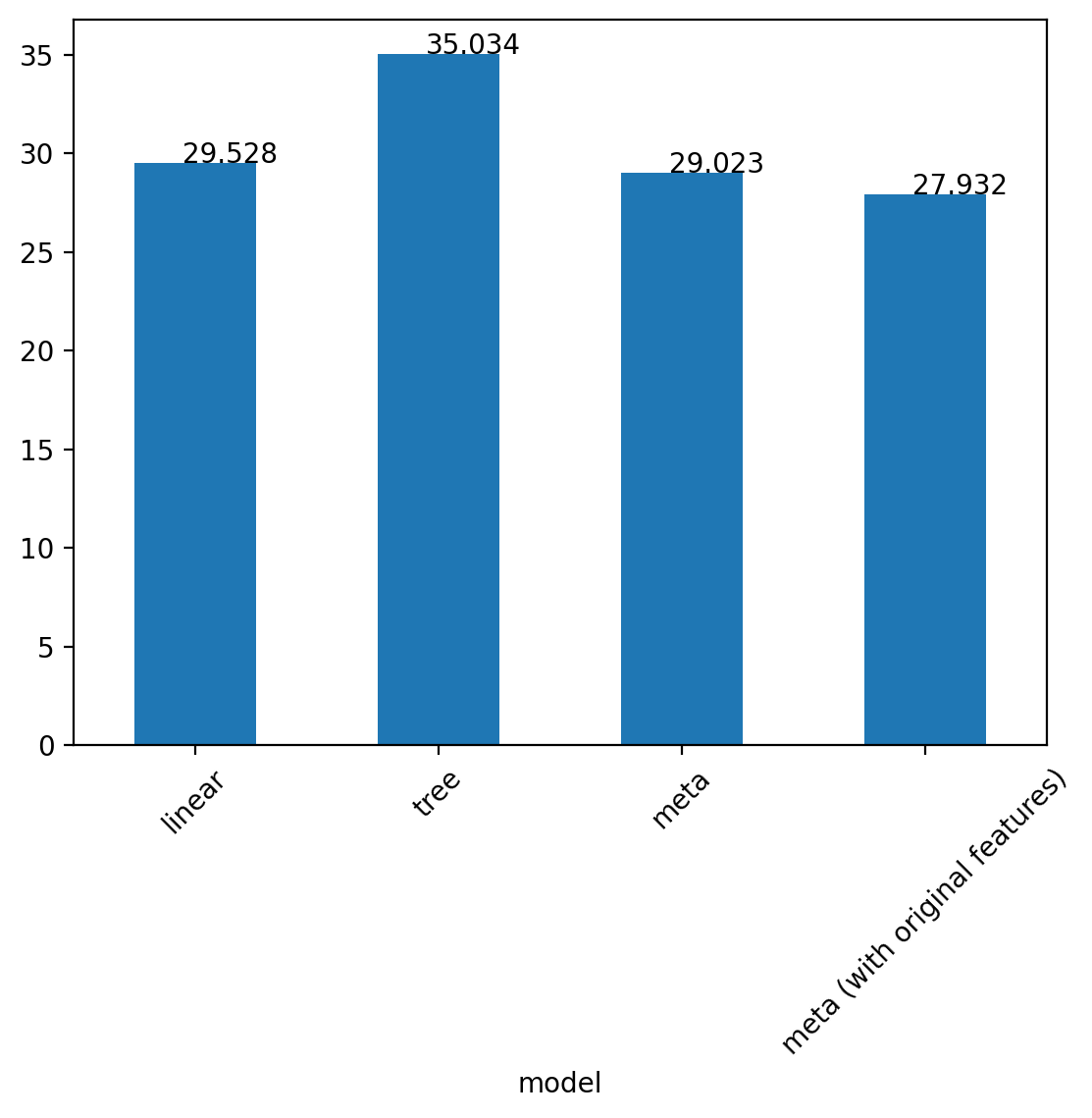
# bar plot for showing the errors for all models

# Create a dataframe with the errors
df = pd.DataFrame({'model': ['linear', 'tree', 'meta', 'meta (with original features)'],
                     'test_error': [mean_squared_error(y_test, lr.predict(x_test.reshape(-1, 1))),
                                    mean_squared_error(y_test, dt.predict(x_test.reshape(-1, 1))),
                                    mean_squared_error(y_test, lr2.predict(x_test_2d)),
                                    mean_squared_error(y_test, lr3.predict(x_test_3d))]})
df.plot(x='model', y='test_error', kind='bar', legend=False, rot=45)
# Put the numbers on the bars
for i, v in enumerate(df.test_error):
    plt.text(i - 0.05, v , str(round(v, 3)))