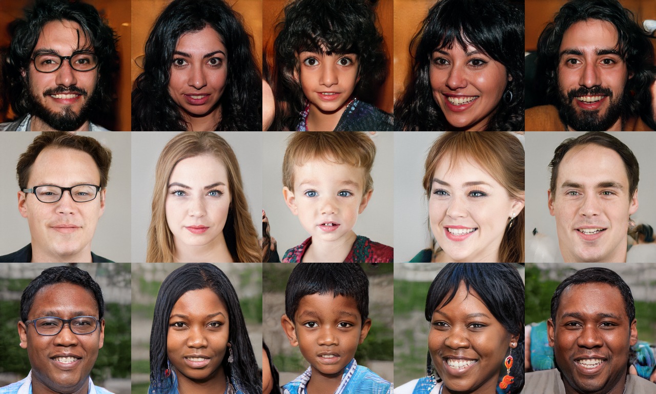
No one. Each face is a random vector of 512 numbers pushed through a trained network.
Karras, Laine & Aila, A Style-Based Generator Architecture for GANs (StyleGAN), 2019 · CC BY-NC 4.0
Your turn to be the judge
Real or generated?
1generated
2real
3generated
4real
5real
6generated
7generated
8generated
9real
10generated
11real
12real
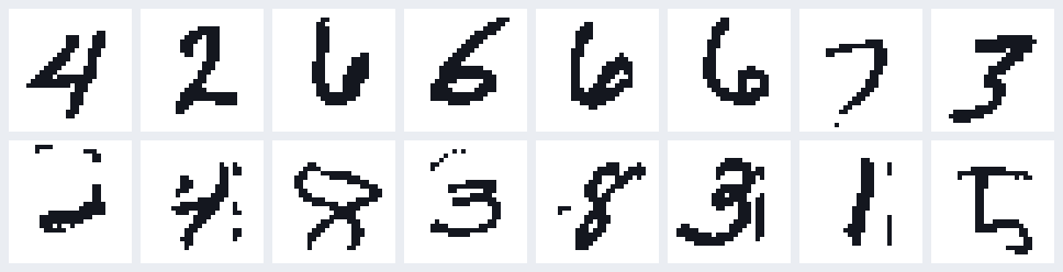
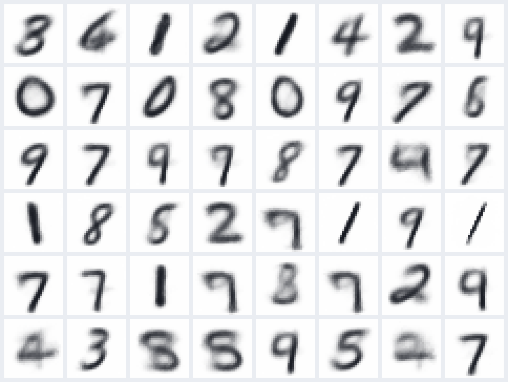
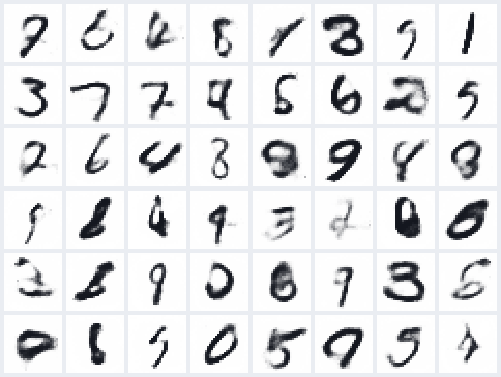
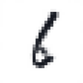
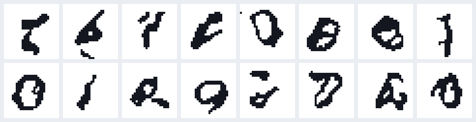
Six are MNIST test digits, six come from a network. Write down which six are fake.
Generated: 1, 3, 6, 7, 8, 10 (teal frames). Six from a small GAN, trained in about 9 minutes: the topic of the next lecture.
Generation is not only "make a random picture"
Predict the output, then look
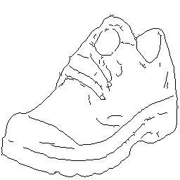
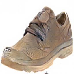
a sketch → a photo
→
?
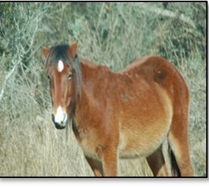
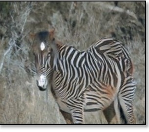
a horse → a zebra
→
?
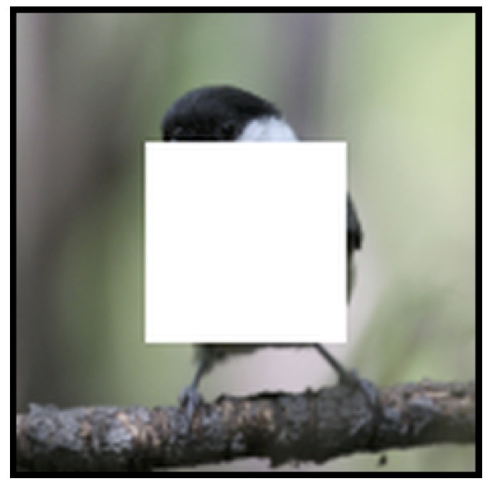
fill a hole
→
?
a label map → a landscape
→
?
What should come out on the right? Is there exactly one right answer?
Each input allows many plausible outputs. A generator must pick one that looks real.
pix2pix (Isola et al. 2017) · CycleGAN (Zhu et al. 2017) · Context Encoders (Pathak et al. 2016) · SPADE (Park et al. 2019). All published model outputs.
One input, many answers
The same label map, three different photographs
the condition
→
sample 1
sample 2
sample 3
A generator does not learn one answer. It learns a distribution of answers and draws from it.
SPADE / GauGAN, Park et al. 2019, teaser figure: here the variation comes from a style image given to the generator.
What all of these share
Randomness in, a learned network, a sample out
Training means: adjust $\theta$ until the samples look like the data. But what is the loss?
What can the condition be?
Tell the generator what you want
a label $c = 7$
our own conditional VAE: eight different random $z$, all asked for a 7
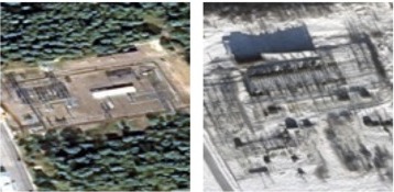
a sentence + a date“a satellite image of an electric substation in Finland”, August vs January
DiffusionSat (Khanna et al., 2024): same caption, only the month changes
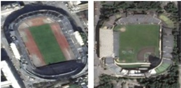
a sentence + a place“a satellite image of a stadium”, France vs USA coordinates
DiffusionSat: same caption, only the latitude and longitude change
an image a sketch, a label map, a photo with a hole
→
pix2pix, from the earlier slide
The condition fixes what; the randomness still decides which one of the many matching outputs you get.
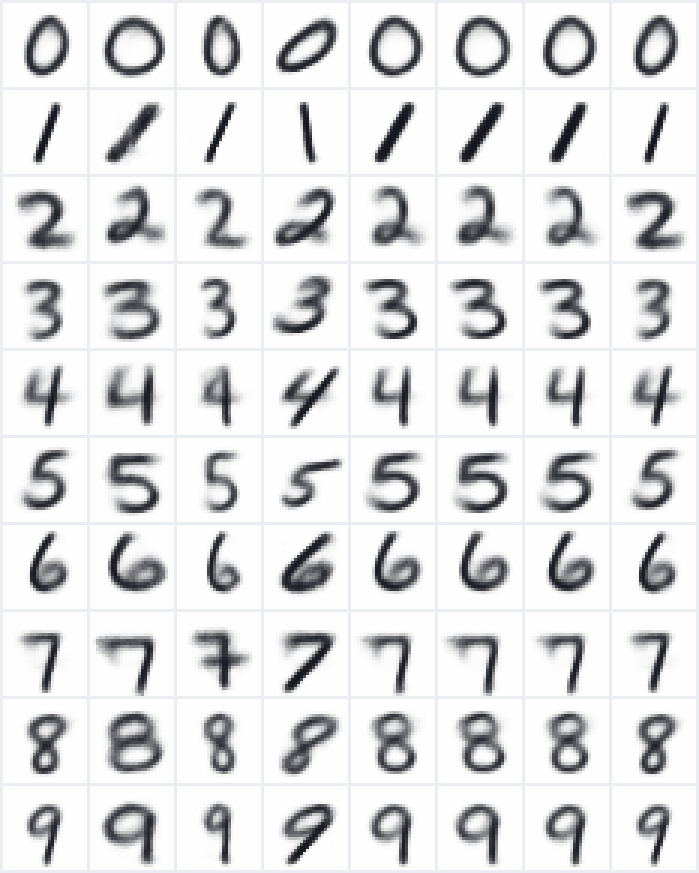
Our conditional VAE, all labels at once
The label picks the digit; the random $z$ picks the style
0123456789
Each row: one label $c$, from 0 to 9.
Each column: one random $z$, the same all the way down.
Read down a column: every digit is written with the same slant and thickness. The code $z$ carries the handwriting; the label carries the identity.
Earlier in this course
You have already built a generator
Our name model reads three characters and gives a probability for every next character.
after a a b, the trained model says:
–
0.46i
0.12h
0.09r
0.08b
0.06s
0.04other 21
0.15
Generate: sample a character, append it, repeat.
a→a→b→i→d→–
A different random draw at any step gives a different name. That is a generative model: it gives probabilities, and we sample from them.
Same idea today: learn a distribution, then sample from it. Only now the samples are images.
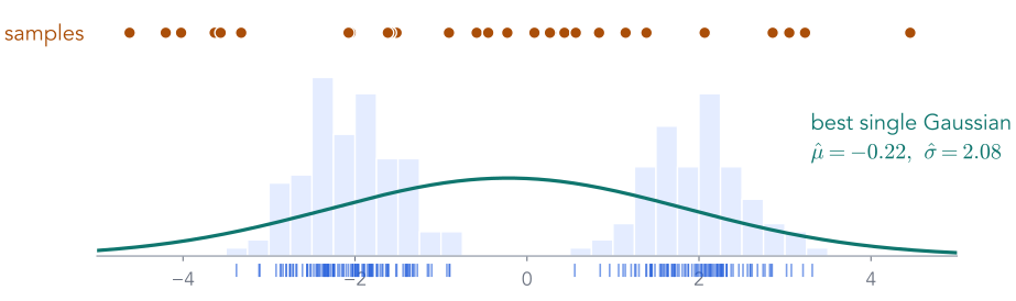
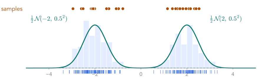
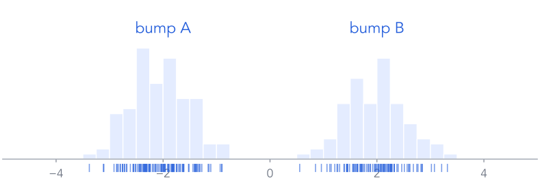
Step 1: pick a bump for each sample, with the learned weights.
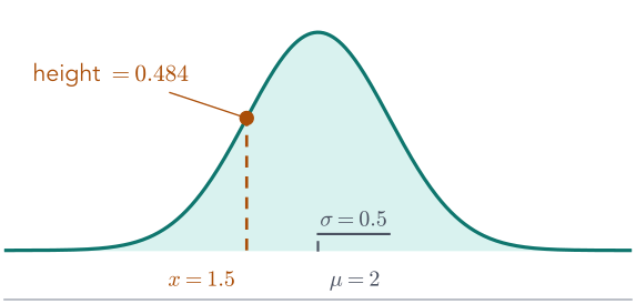
Step 2: draw a number from that bump: its centre plus its width times standard noise.
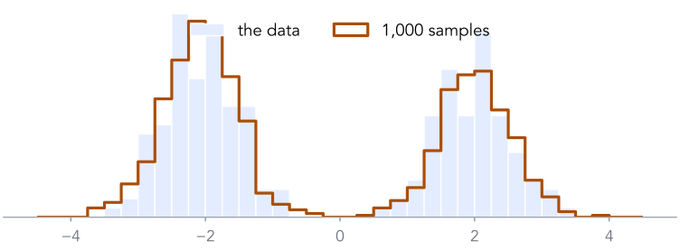
1,000 new numbers that follow the data, and none of them is a copy of a training number.
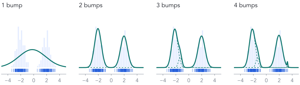
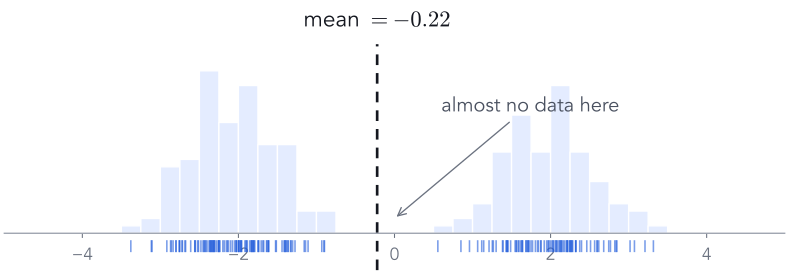
But how many bumps should we fit?
More bumps always fit the training data better
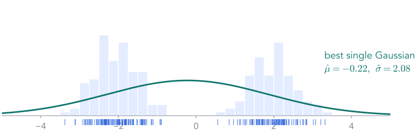
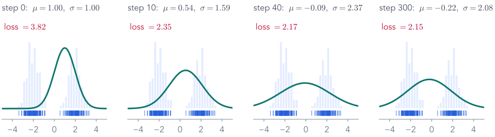
1, 2, 3, 4 bumps, each fitted with the same loop. The training score rises every time. So which one do we keep?
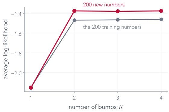
Score on data the fit has never seen
New data decides: two bumps
Draw 200 new numbers from the same hidden recipe and score each fit on them.
1 → 2 bumps: $−2.153 \to −1.376$ per number. A real improvement.
3 or 4 bumps: the training score creeps up, the new-data score does not. The extra bumps fit noise in the 200 training numbers.
Choose the size of a model by how well it scores data it has not seen. That holds for bumps, and for networks.
Step 1 · Learn, looked at closely
Hidden in the fit: which bump made each point?
If we knew the coin for every point
fitting is easy: average the A-points for bump A's centre, the B-points for bump B's.
We don't, so ask for each point
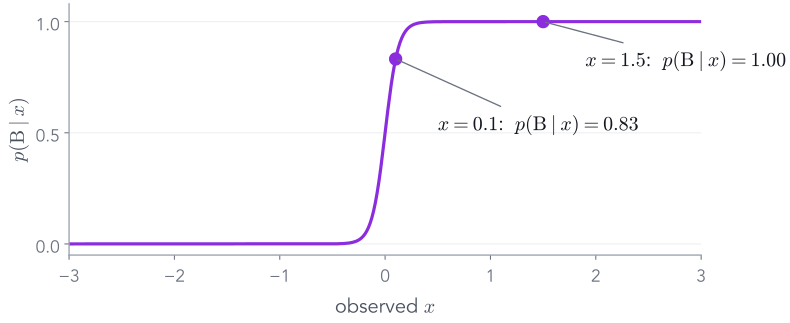
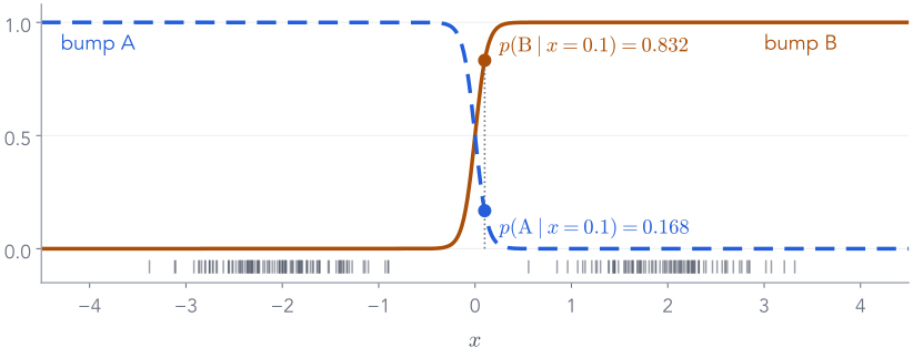
given this $x$, how probable is it that bump B made it? That is $p(\mathrm{B}\mid x)$.
Running the story backwards, from a number to its likely hidden cause, is called inference. The gradient descent we just ran was doing it all along: four slides on, we will see where.
Bayes' rule is just this table: multiply, then divide by the total. Note the total is exactly the $p(x)$ of the two-bump formula.
Do it for every $x$
The backwards step, as a curve
Repeat the table for every $x$ and plot $p(\mathrm{B}\mid x)$.
Far right: certainly B. Far left: certainly A. Near 0: unsure.
For these two bumps the curve is exactly $\mathrm{sigmoid}(16x)$: a logistic regression in disguise.
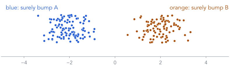
These are the colours on the 200 points two slides ago.
The backwards step, in one line
Posterior = softmax of (log prior + log likelihood)
log_joint = log_softmax(logits) + Normal(means, log_sd.exp()).log_prob(x) # [K]posterior = softmax(log_joint) # divide by the total: Bayes
With the fitted bumps, at $x = 0.1$: $p(\mathrm{A}\mid x) = 0.094$, $p(\mathrm{B}\mid x) = 0.906$. (With the true recipe it was 0.832: the fitted bumps are slightly different.)
Softmax is "exponentiate, then divide by the total": exactly the last column of the Bayes table.
Why learning needs the backwards step
The gradient of $\log p(x)$ is weighted by the posterior
At $x = 0.1$: bump B's centre is pulled by $0.832 \times (0.1 - 2)/0.25 = −6.32$, bump A's by $0.168 \times (0.1 + 2)/0.25 = 1.41$.
Each point pulls each bump in proportion to how likely that bump made it. Learning needs the posterior for every point: a 2-row table here, an intractable patch for images.
Four words for the rest of the lecture
Prior, likelihood, evidence, posterior
name
symbol
question it answers
at $x = 0.1$
prior
$p(z)$
what do we believe about $z$ before seeing $x$?
0.5, 0.5
likelihood
$p(x\mid z)$
if $z$ were known, how probable is this $x$?
$5.84\times 10^{-4}$ for B
evidence
$p(x)$
how probable is $x$ overall, summing over $z$?
$3.51\times 10^{-4}$
posterior
$p(z\mid x)$
having seen $x$, which $z$ explains it?
B: 0.832
Generating uses the prior and the likelihood. Learning needs the evidence and the posterior.
Part 1, second half
The same recipe, on real images
Learn a distribution, then sample from it: can Gaussian bumps generate handwritten digits? How far does this simple toolkit get us, and where does it run out?
The plan, as a picture
Squeeze, fit bumps, sample, un-squeeze
Two questions before any code: each bump is a Gaussian over what? And how many bumps?
Which dimension is each Gaussian?
One bump, three possible sizes
each bump is a Gaussian over
centre
covariance
numbers per bump, with its weight
1 number (the toy)
1
1 (a width)
3
784 pixels, every pixel on its own
784
784 widths
1,569
784 pixels, with all pixel pairs
784
307,720
308,505
50 PCA numbers (what we fit)
50
1,275
1,326
Samples from one 784-pixel Gaussian with independent pixels: each pixel jitters on its own, so you get static around the average digit. Strokes need pixels that move together.
Keep the covariance, shrink the dimension: a full Gaussian over 50 numbers costs about 230 times less than one over 784 pixels.
The squeeze, and the way back
PCA and inverse PCA: generation needs both
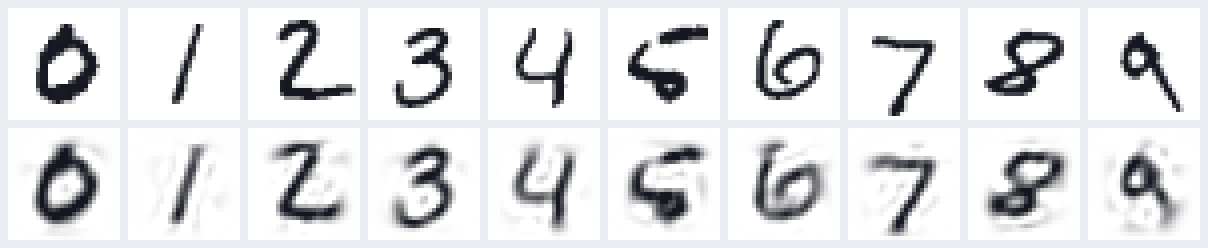
PCA, image to $d$ numbers: coordinates along the $d$ directions in which digits vary most.
Inverse PCA, $d$ numbers back to an image: add the directions back onto the mean digit.
$$\underbrace{\hat x}_{784} = \bar x + \underbrace{V}_{784\times d}\,\underbrace{z}_{d}$$
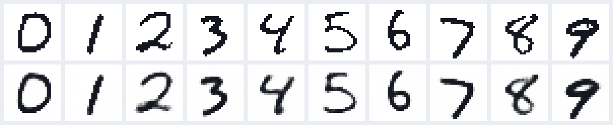
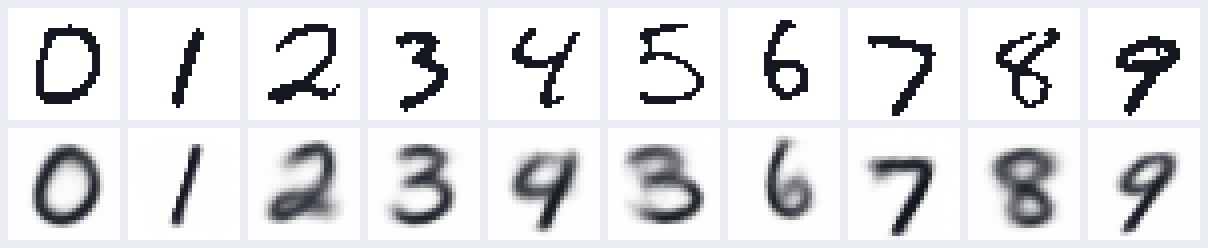
top: test digits, our 3 among them · bottom: PCA to 50 numbers, then inverse PCA
The bumps only ever see $z$. Every generated sample is $d$ numbers until the inverse PCA turns it into pixels. With $d = 50$, 82.5% of the variation survives the round trip.
Squeeze all the way to 2 numbers
In 2-D you can see every bump
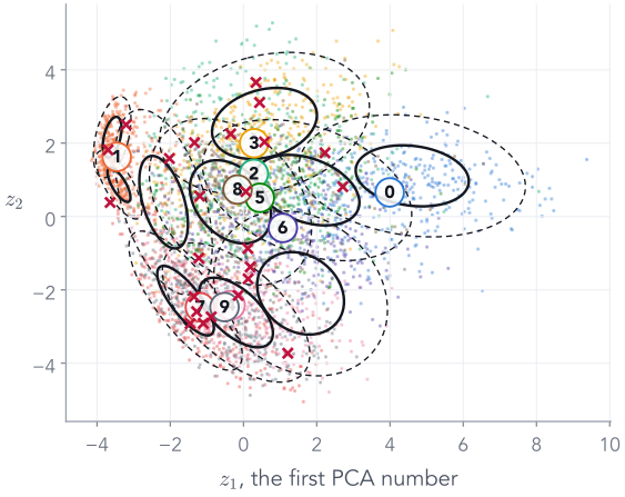
4,000 test digits by their 2 PCA numbers, coloured by label (the model never saw labels). Black: 10 fitted bumps, 1 and 2 widths. Red ×: 24 samples.
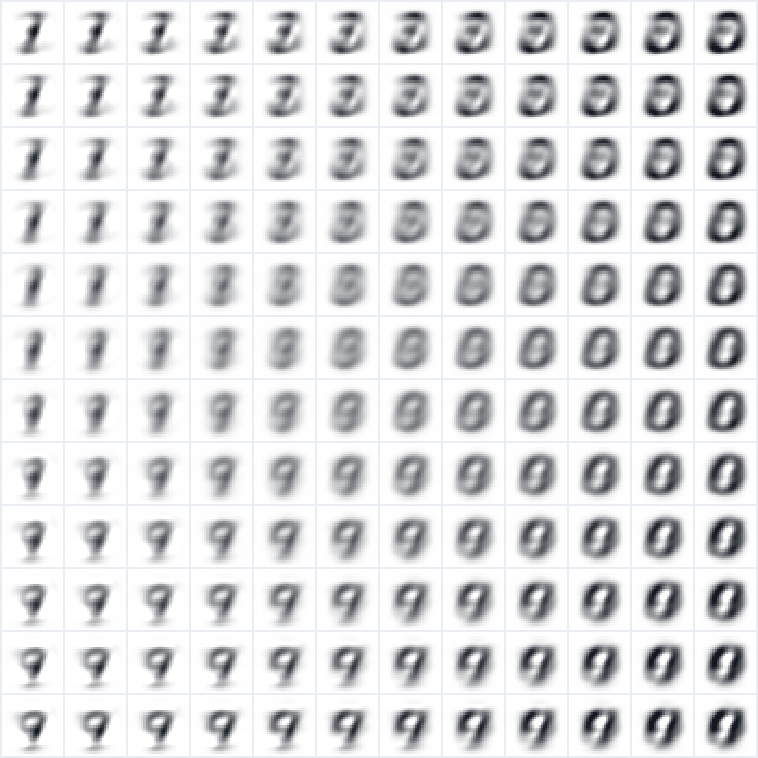
Inverse PCA of a grid over the plane: every point is a blend of a few blurry shapes.
the 24 red × after inverse PCA
2 numbers keep only 16.8% of the variation. Every bump is visible, every sample is a ghost: interpretable is not the same as good.
PCA: one SVD gives the directions; each image becomes $d$ numbers.
The mixture:logits [K], means [K, d], L [K, d, d] lower-triangular, so each covariance $LL^\top$ is always valid.
Learning: the loop that fitted the two bumps, unchanged: minus the average log-probability, Adam.
Generating: pick a bump by its weight, draw $d$ numbers from it, inverse PCA to 784 pixels.
Try it: every combination below was fitted
Slide the dimension and the number of bumps
variation kept by $d$ numbers: 82.5% parameters: 132,599 score on new images: −16.5 new images prefer $K$ = 100 at this $d$
test digits
after PCA to $d$ numbers and back
24 samples from the $K$-bump fit, after inverse PCA
How many bumps for MNIST?
The toy's rule: score on images the model has not seen
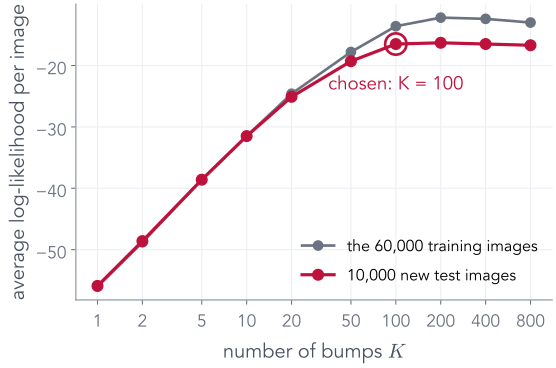
$d = 50$. Fit $K$ = 1, 2, 5, 10, 20, 50, 100, 200, 400, 800 bumps to the 60,000 training images.
Training images: more bumps fit them better, as with the toy.
10,000 new test images: the score stops improving at $K = 100$. Doubling to 200 bumps changes the score by +0.2 nats. At 800 even the training score drops: that many bumps are more than 2,000 steps can fit.
Pick the smallest $K$ that does as well as any on new images: $K = 100$, 132,599 parameters, each bump a Gaussian over 50 numbers.
Choosing $K$ without held-out images
AIC and BIC: charge for every parameter
$$\mathrm{AIC} = 2p - 2\log L \qquad\qquad \mathrm{BIC} = p\,\log N - 2\log L$$
$\log L$: the training log-likelihood, summed over all $N$ = 60,000 images · $p$: the number of parameters · smaller is better
rule
needs
price per parameter
picks
score on new images
10,000 extra images
none, it is measured
$K = 100$
AIC
training data only
2
$K = 100$
BIC
training data only
$\log 60{,}000 = 11.0$
$K = 50$
New images and AIC agree on $K = 100$; BIC, which charges more per parameter, keeps only 50. With plenty of data, measure on new data; with little, AIC or BIC.
What the bumps learned
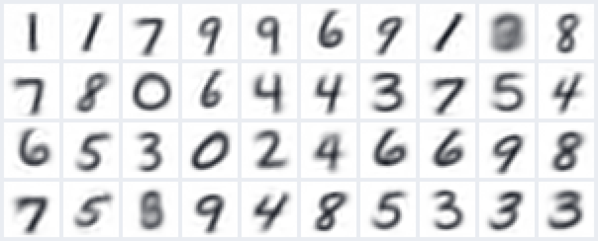
Each bump's centre is a style of digit
the centres of the 100-bump fit, after inverse PCA, heaviest bump first (the heaviest has weight 3.9%)
The hidden coin now has 100 sides, one prototype each, found without the labels. The backwards step $p(z\mid x)$ is still just a 100-row table.
Step 2 · Generate
Samples, as the number of bumps grows
1 bump: a single Gaussian over the 50 numbers of every digit
10 bumps
100 bumps, the size chosen on new images
Or skip PCA: model the 784 pixels directly
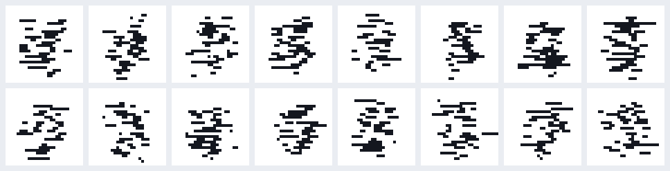
A mixture of Bernoullis: each bump is 784 ink probabilities
the 20 heaviest of 200 bumps: $\pi_k$, ink probability per pixel
samples: pick a bump, flip each pixel's coin
Inside a bump every pixel is on its own, so samples are speckled; only the choice of bump ties pixels together. Same lesson as the 784-pixel Gaussian.
An honest look
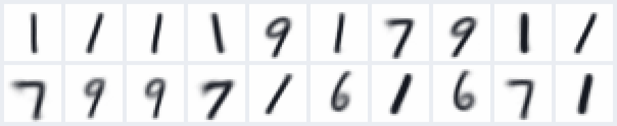
New digits, not copies, and not yet sharp
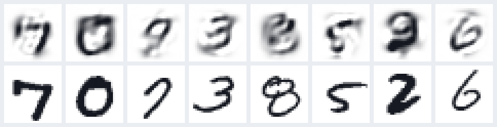
top: 8 samples · bottom: the closest of the 60,000 training images
What worked
The Part 1 loop, unchanged, learns a distribution over images and samples digit-like shapes, close to real digits but not copies of them.
What did not
Blur from the straight-line squeeze, and each bump can only stretch its template along fixed directions, not bend a stroke.
Why we cannot stop here
This recipe does not scale
image
numbers
covariance per bump
MNIST, 28 × 28 grey
784
307,720
32 × 32 colour
3,072
4.7 million
64 × 64 colour face
12,288
75.5 million
256 × 256 colour photo
196,608
19.3 billion
Squeeze first? A straight-line squeeze needs more and more numbers for richer images, and still blurs.
More bumps? Each bump is one template plus a Gaussian wiggle. Every pose, style and lighting needs its own templates.
Nothing is shared: the bump for a slanted 7 learns nothing from the bump for an upright 7.
We need a squeeze that can bend, learned by a network, and parts that are shared. Part 2: the autoencoder.
End of Part 1
What we did, and what comes next
What we did
Learn = choose parameters that make the data probable.
Generate = sample from the learned model.
One bump was too simple; a hidden coin $z$ fixed it.
Scoring $x$ sums over $z$; learning needs the backwards step $p(z\mid x)$.
In code: one loop, loss = -log_p(x).mean(); choose the size on new data.
On MNIST: PCA to 50 numbers, 100 Gaussian bumps over them, inverse PCA: digit-like samples, but blurry, and the recipe does not scale.
Next: images
PCA squeezed each image along straight lines. Next, learn the squeeze with a network: encode each image into a few numbers and rebuild it. That is the autoencoder.
Part 3 returns to this probabilistic story, with a code $z$ in place of the coin.
Part 2 of 7
From PCA to the autoencoder
Part 1 ended with PCA: squeeze an image to a few numbers along straight lines, then rebuild it. An autoencoder learns the squeeze with a network instead, so it can bend. First, the bridge: PCA is already one.
✓Distributions and fitting
2Autoencoders
3The probabilistic view
4KL divergence
5Variational inference and the ELBO
6Reparameterisation
7The VAE on MNIST
The bridge from Part 1
PCA was an autoencoder all along
Train the straight-line version by gradient descent
error: squared error per test image, summed over 784 grey pixels · last column: 1 means the decoder spans exactly PCA's directions
Gradient descent finds exactly PCA's error and PCA's directions. Only the individual vectors may differ: any rotation of the same directions rebuilds just as well.
Now let it bend
Same 2 numbers, add layers and ReLUs
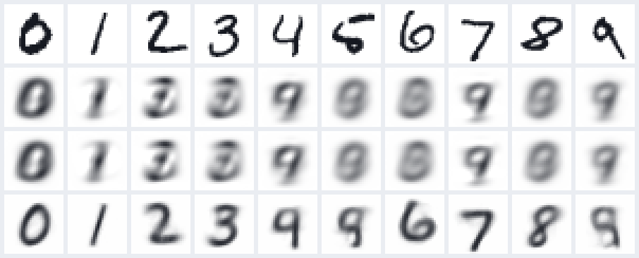
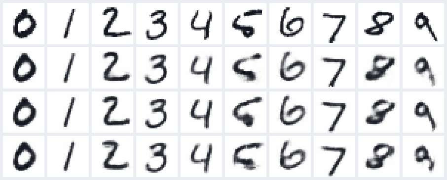
rows: test digits · PCA · linear autoencoder · MLP autoencoder, each squeezing to 2 numbers
error
$d = 2$
$d = 16$
PCA
43.6
21.1
linear AE
43.6
21.1
MLP AE
29.3
7.6
With only 2 numbers, the straight-line squeeze keeps a blurry average; the bendy one keeps which digit it was. Same idea, more flexible maps.
for every code unit $h_j$ and every pixel $x_i$: how much does $h_j$ change if $x_i$ changes a little? Add up the squares.
What it buys
two slightly different 3s get almost the same code. Nearby inputs, nearby codes: a first step towards a smooth code space.
What autoencoders are used for
Compress, clean, search, and spot the odd one out
Compress: 784 pixels → 16 numbers, 49× fewer.
Clean: the denoising slide.
Search: similar images have nearby codes, so search the codes.
Spot anomalies: an image the model has never seen anything like gets a large reconstruction error.
top: typical test digits, loss ≈ 40.5
bottom: the 8 worst of 10,000, loss up to 218.0
Useful, all of it. But none of it generates a new image. Can the decoder do that on its own?
Part 2, second half
Can an autoencoder generate?
The decoder turns codes into digits. If we pick a code ourselves, do we get a new digit?
The obvious idea
Keep the decoder, feed it a random code
The decoder turns codes into digits. So a random code should give a random digit. Right?
What is a "random code"?
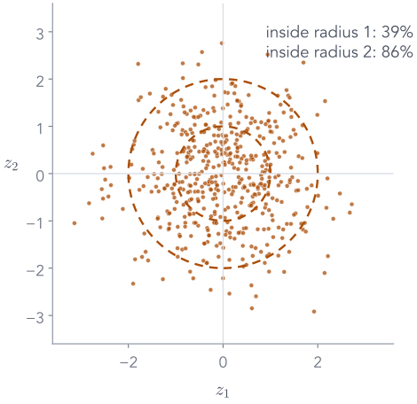
$z \sim \N(0, I)$: two independent bell curves
Draw $z_1$ from a standard bell curve $\N(0, 1)$: mean 0, spread 1. Draw $z_2$ the same way, independently.
Together that is written $\N(0, I)$: the 0 says the centre is $(0, 0)$; the I (identity matrix) says each number has spread 1 and the two do not depend on each other.
500 draws, plotted: most land within 2 of the origin, almost none beyond 3.
Why this choice? It is the simplest distribution we can sample from. The decoder, though, was never told about it.
What actually comes out
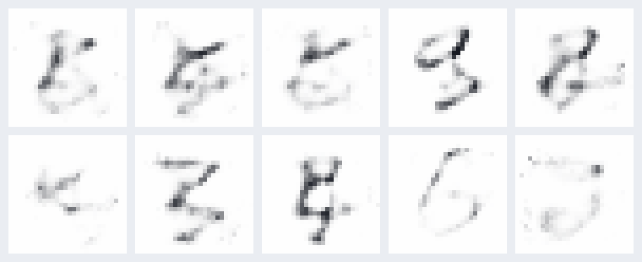
Random codes give scribbles
ten codes drawn from $\N(0, I)$ in 16 dimensions, through the trained decoder
The decoder only ever saw codes made by the encoder. Where do those codes live?
Look inside (2-number version)
Where 5,000 test digits land
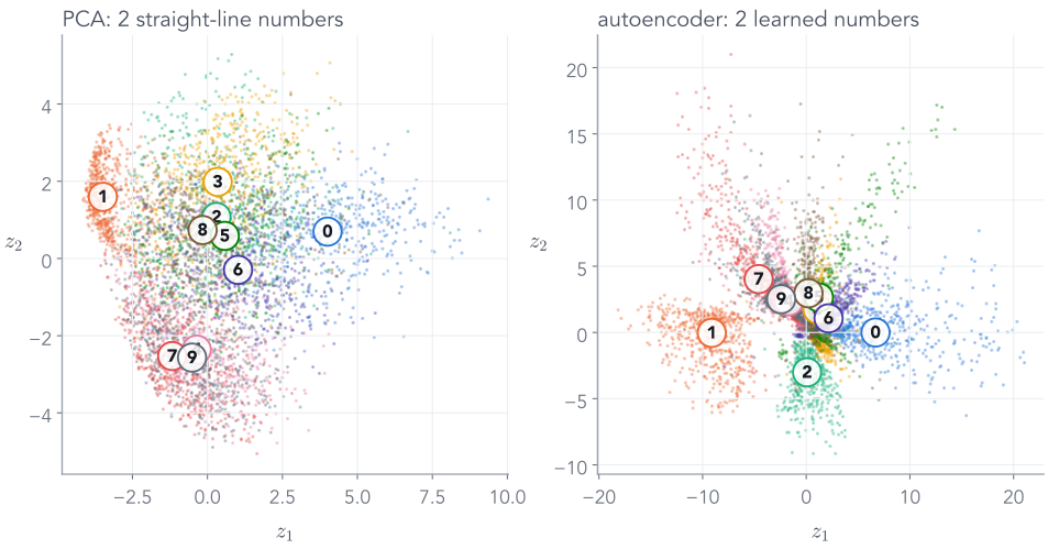
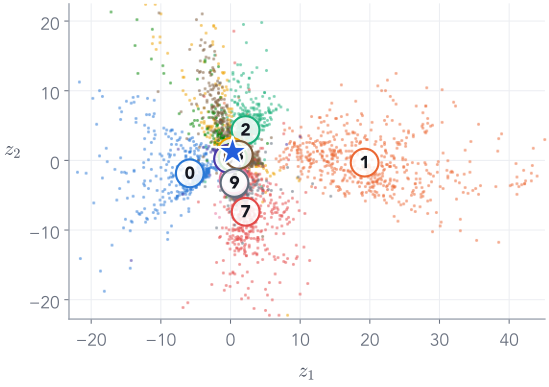
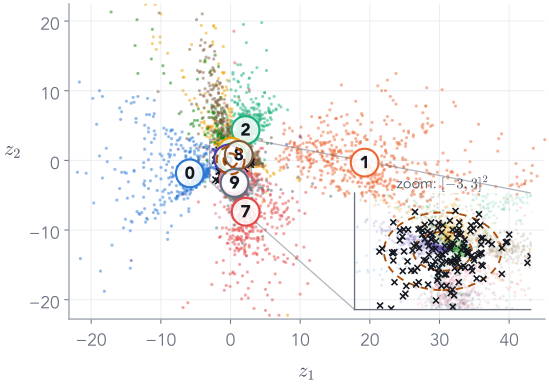
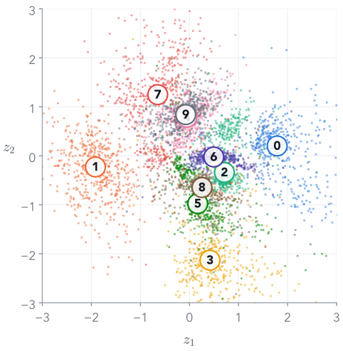
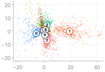
Each dot is one test digit's code, coloured by its true label. The star is our 3.
Same digits cluster together. Nobody asked for that; it just helps reconstruction.
Look at the axes: $z_1$ runs from −18.5 to 40.4, $z_2$ from −19.7 to 19.4. Nothing made the codes stay near the origin.
The code space has an arbitrary shape, scale and position.
Overlay random codes
Random draws all land in one small spot
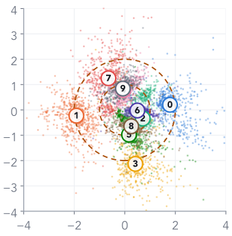
Now add 150 random codes from $\N(0, I)$ (black ×), the kind we fed the decoder two slides ago. Dashed circles: radius 1 and 2. On this map they all fall into one small crowded patch (zoomed, bottom right).
ten of them decoded: some digits, some smudges
And we can never generate a 1: the 1s live near $z_1 \approx 20$.
To sample, we need to know where the codes are, and every point there must decode to something sensible.
Try it: the trained autoencoder, in your browser
Pick a code, any code, and decode it
decoded from $z$the real digit
$z$ = (, )
A real digit's code decodes well. A random code usually gives a smudge: the decoder only learned the dotted regions.
Part 1's tool, on the autoencoder's codes
Fit bumps to where the codes actually are
random codes from $\N(0, I)$, decoded by a 16-number autoencoder
50 Gaussian bumps fitted to the autoencoder's 16 numbers, sampled, decoded
Bolting a density onto the codes works, and a better squeeze gives better samples. The VAE goes one step further: it shapes the codes during training, so that $\N(0, I)$ itself is the right density.
What we want instead
Encode to a cloud, not a point
Known: pull every cloud towards $\N(0, I)$, so random draws land on real codes.
Smooth: every point in a cloud must decode to that image, so neighbourhoods are meaningful.
A preview of where we are going
The same plot for a VAE
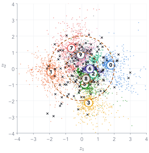
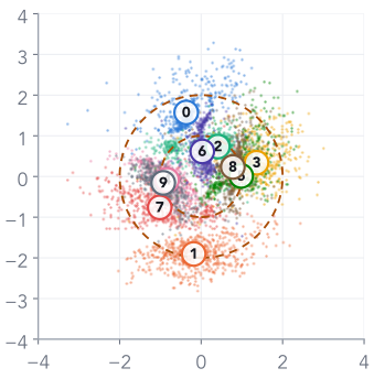
Same data, same 2-number code, same random draws. Now the codes sit inside $\N(0, I)$.
the same kind of random codes, decoded
To get here: make the model probabilistic (Part 3), measure how close two distributions are (Part 4), and derive the loss (Part 5).
End of Part 2
What we did, and what comes next
What we did
An encoder squeezes an image into a short code; a decoder rebuilds it. The image is its own target.
Random codes from $\N(0, I)$ decode to scribbles.
The codes spread over an arbitrary range, and the decoder never saw the space between them.
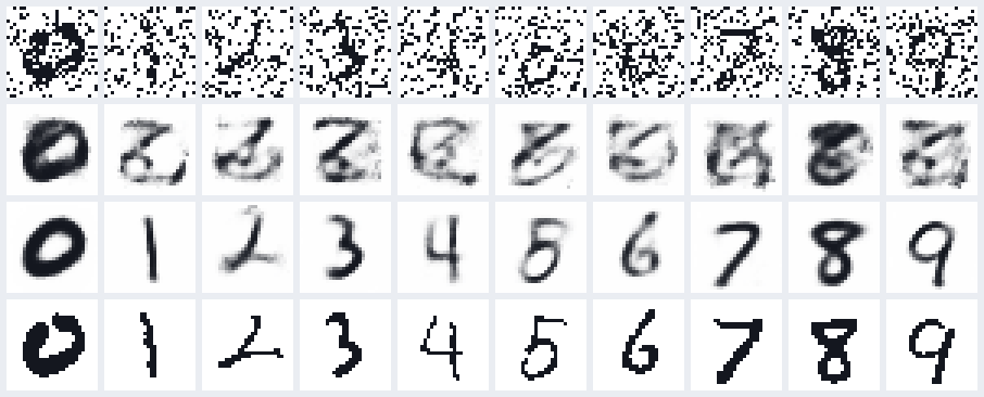
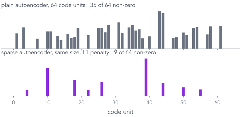
Variants change the input (denoising) or add a penalty (sparse, contractive).
The wish: encode each image to a cloud, and keep every cloud near $\N(0, I)$.
Next: the probabilistic view
Turn the decoder into a probability model with a prior over codes, and ask what it would take to train it by maximum likelihood, as in Part 1.
Part 3 of 7
The probabilistic view: a decoder is a likelihood
The autoencoder could not generate because nothing said where codes live. Part 1 had exactly what is missing: a prior over the hidden choice. Put Part 1's story and Part 2's decoder together.
✓Distributions and fitting
✓Autoencoders
3The probabilistic view
4KL divergence
5Variational inference and the ELBO
6Reparameterisation
7The VAE on MNIST
From a coin to a code
Same story, bigger pieces
two bumps (so far)
images (from now on)
hidden $z$
a coin: A or B
2 real numbers $(z_1, z_2)$, drawn from $\N(0, I)$
$p(x\mid z)$
a bump at $-2$ or $+2$
a neural network, the decoder, with weights $\theta$
observed $x$
one number
784 pixels, each ink (1) or paper (0)
sum over $z$
2 terms
every point in a plane: infinitely many
Next three slides: generate one image this way, one step at a time.
Generating an image · step 1 of 3
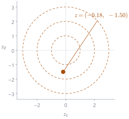
Draw a code
$$z \sim \N(0, I)$$
Two numbers, each from a standard bell curve: like flipping the coin, but the "coin" can land anywhere in the plane.
This draw: $z = (−0.18,\ −1.5)$.
On its own, $z$ means nothing. The decoder will give it meaning.
Generating an image · step 2 of 3
Decode it into 784 pixel probabilities
$\pi_i$ is the probability that pixel $i$ is ink. Dark grey = probably ink; white = probably paper.
Generating an image · step 3 of 3
Flip one coin per pixel
probabilities $\pi$
→
one sample $x$
$$x_i \sim \mathrm{Bernoulli}(\pi_i)$$
Each pixel independently: ink with probability $\pi_i$.
That is a generated image. In practice we usually display $\pi$ itself, because it looks cleaner.
The same two steps as before
Generating is easy. Learning is the catch.
Generate ✓
draw $z \sim \N(0,I)$, decode, flip pixels. Three slides, done.
Learn ?
choose the decoder's weights $\theta$ to make the training images probable:
2 numbers per code, so we can afford a 901 × 901 grid of decoder calls: $\log p_\theta(x) = −128.7$ nats.
Why not just compute $p_\theta(x)$?
The integral is intractable
No formula. With two bumps, $p(x)$ was a sum of 2 terms. Here it is $\int p(z)\,p_\theta(x\mid z)\,dz$ with a neural network inside: no algebra gives the answer.
Too many terms to add up. Put a grid of 901 points on every axis of the code and add up the decoder's answers:
"Intractable" means exactly this: no formula, and far too many terms to sum.
numbers in $z$
decoder calls
1
901
2 (our 3)
$8.1\times 10^{5}$ · a second
4
$6.6\times 10^{11}$ · a week
8
$4.3\times 10^{23}$
16
$1.9\times 10^{47}$
And we need $p_\theta(x)$ for every image, at every training step.
Idea: estimate the integral by sampling
Random codes almost never hit the right patch
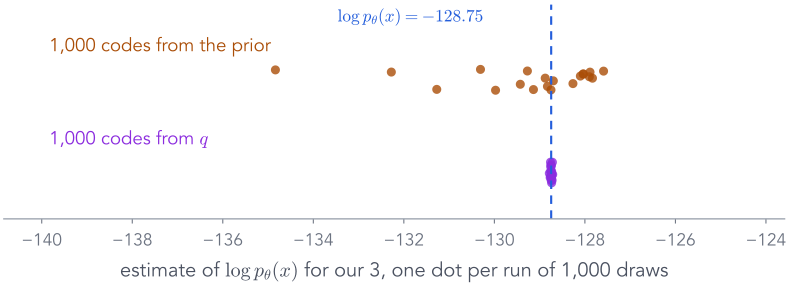
$$p_\theta(x) = \underbrace{\E_{z\sim p(z)}\big[\,p_\theta(x\mid z)\,\big]}_{\text{the average over codes from the prior}} \approx \frac1S\sum_{s=1}^{S} p_\theta(x\mid z_s)$$
100,000random codes $z_s\sim\N(0,I)$
0.07%land within 2 widths of our 3's patch
−363.9median $\log p(x\mid z)$ of a random code
−121.0the best of the 100,000: $\log p(x\mid z)$
A typical random code makes our 3 about $e^{243}$ times less probable than the best code. Blind sampling wastes almost every draw.
Inference, like the coin and the bumps
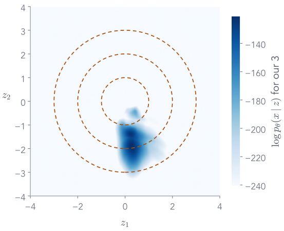
The backwards step: which codes could have made our 3?
Part 1's Bayes table, with a plane of codes instead of two bumps:
The bottom is the evidence: the same impossible integral. So the posterior is out of reach too.
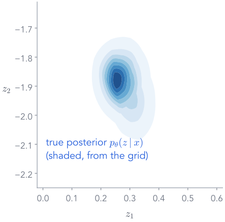
From the 2-number grid we can still look at it: a small, slightly tilted patch near $(0.25,\ −1.88)$, about 0.05 wide. The prior is 1 wide: one image pins its code down tightly.
Training needs this patch for every image. Next: three ways to approximate a posterior we cannot compute.
When the posterior cannot be computed, approximate it
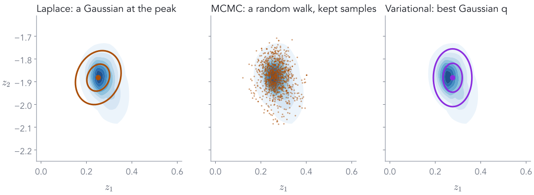
Three ways, all run on our 3's real posterior
Laplace: find the peak, fit a Gaussian to the curvature there. Fast, local.
MCMC: a random walk that visits regions in proportion to the posterior. Exact in the long run, slow.
Variational: choose a simple family $q$ and optimise it to be as close as possible. Fast, trainable.
Today: only the variational one. It turns inference into optimisation, which is what neural networks are good at.
The variational idea, for our 3
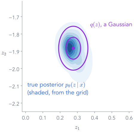
Propose a simple $q$, then pull it towards the true posterior
Four numbers to choose: a centre $m = (m_1, m_2)$ and two widths $s_1, s_2$.
Goal: make $q(z)$ as close as possible to $p_\theta(z\mid x)$, the shaded patch.
"As close as possible" needs a number for how far apart two distributions are.
That number is the KL divergence: the first thing in Session 2.
End of Part 3 · end of Session 1
What we did, and what comes next
What we did
Learn = make the data probable; generate = sample. Code: one loop.
Autoencoders compress and rebuild (plain, denoising, sparse, contractive), but cannot generate.
As a probability model: prior $p(z) = \N(0, I)$, likelihood $p_\theta(x\mid z)$ from the decoder.
Training needs $p_\theta(x)$ and the posterior $p_\theta(z\mid x)$: both intractable.
Variational idea: a simple $q$, pulled close to the posterior.
Session 2
A distance between distributions (KL), the loss that pulls $q$ close without ever computing $p_\theta(x)$ (the ELBO), gradients through random draws, and the VAE on MNIST.
Session 2 · where we stopped
Last time: we need $q$ close to a posterior we cannot compute
A decoder plus a prior is a probability model: $p(z)\,p_\theta(x\mid z)$.
Training it needs $p_\theta(x) = \int p(z)\,p_\theta(x\mid z)\,dz$: intractable.
So does the posterior $p_\theta(z\mid x)$, the shaded patch for our 3.
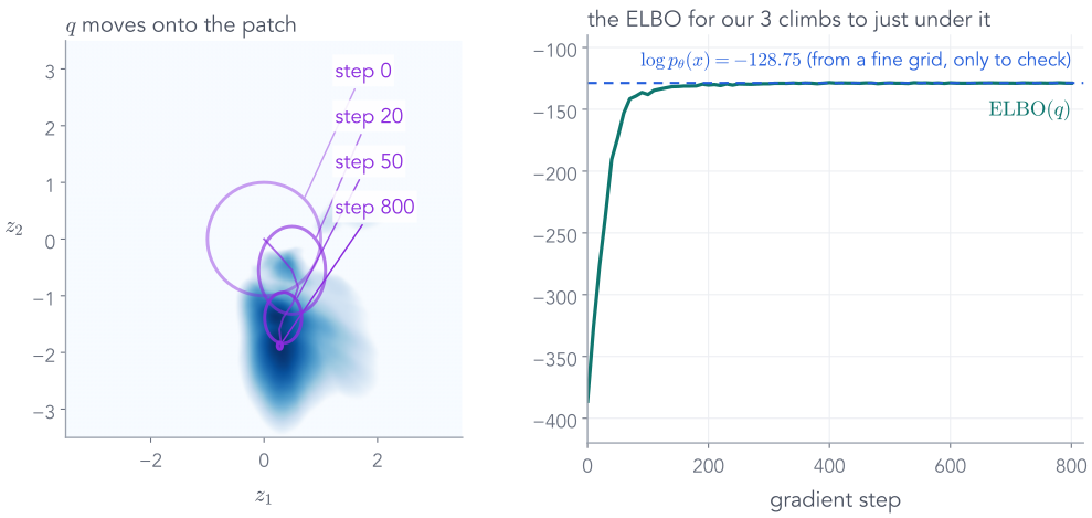
Variational idea: a simple Gaussian $q$ (purple), pulled close to it.
The VI lecture's two lines: $\log p(D) = \ELBO(q) + \KL\big(q\,\|\,p(\theta\mid D)\big)$ for every $q$ $z = \mu + \sigma\cdot\eps$: a random draw with a gradient
Today: those two lines for our 3, then one network that applies them to every image: the VAE.
Part 4 of 7
KL divergence, recalled for our 3's code
We want $q$ close to the posterior. The VI lecture built "close" from scratch (its Part 2). Here: the facts we need from it, and the one formula every VAE loss uses, a cloud against the prior $\N(0, I)$.
✓Distributions and fitting
✓Autoencoders
✓The probabilistic view
4KL divergence
5Variational inference and the ELBO
6Reparameterisation
7The VAE on MNIST
From the VI lecture, Part 2
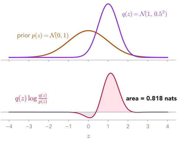
KL is an average of log-ratios, under its first argument
A code with several coordinates and a diagonal $q$: one such term per coordinate, added. Moving a centre costs $\tfrac12\mu^2$; a width other than 1 costs $\tfrac12(\sigma^2 - 1 - \log\sigma^2)$.
From the VI lecture: $\KL(q\|p)$ is an average under $q$, never negative, not symmetric.
VI minimises $\KL(q\,\|\,\text{posterior})$ because we can draw from $q$; $q$ seeks a mode.
Against the prior: $\tfrac12(\mu^2+\sigma^2-1-\log\sigma^2)$ per coordinate, added.
Next: make $q$ close to the posterior
$\KL(q\,\|\,p_\theta(z\mid x))$ contains the intractable $p_\theta(x)$. The VI lecture's ELBO removes it; Part 5 runs it on our 3, then hands the job to an encoder.
Part 5 of 7
Variational inference for our 3, then for every image
The VI lecture turned "make $q$ close to the posterior" into a loss we can compute, the ELBO, and fitted a coin with it (its Part 6). Here the unknown is our 3's code: run the same loss on it, read the numbers, and see why doing this image by image leads to an encoder.
✓Distributions and fitting
✓Autoencoders
✓The probabilistic view
✓KL divergence
5Variational inference and the ELBO
6Reparameterisation
7The VAE on MNIST
From the VI lecture, Part 6, with an image in place of the coin
Our 3, two choices of $q$. The right end, $\log p_\theta(x)$, is fixed by the model; it does not move when $q$ changes.
$q = \N(0, I)$, the prior
ELBO−386.2
$\log p_\theta(x)$−128.75
gap = KL to the posterior: about 257 nats
$q$ after variational inference (next slides)
ELBO −128.83 · gap 0.08the two points overlap
The total cannot move, so raising the ELBO must shrink the KL: maximise the ELBO and $q$ approaches the posterior, without ever computing $p_\theta(x)$.
$$\ELBO = \underbrace{\E_{z\sim\cenc q}\big[\cdec{\log p_\theta(x\mid z)}\big]}_{\text{rebuild } x \text{ from codes in its cloud}} \;-\; \underbrace{\closs{\KL\big(q(z)\,\|\,p(z)\big)}}_{\text{keep the cloud near } \N(0,I)}$$
First term: the autoencoder's reconstruction score, with the code drawn from the cloud.
Second term: the Gaussian KL to the prior from Part 4, in closed form.
The two wishes from the end of Part 2, derived rather than invented: rebuild well, and keep codes where the prior can find them.
$q$ always depended on the image; now we write it $q_\varphi(z\mid x)$: the best Gaussian under the ELBO, predicted by a network.
"Autoencoder"
image → encoder → code → decoder → image: the shape from Part 2, now with a cloud for a code.
Trained together
Pushing on $\theta$ raises the ELBO mostly by making the data more probable: a better model. Pushing on $\varphi$ shrinks the gap: a better $q$.
Kingma & Welling (2014) and Rezende et al. (2014): one network for the likelihood, one for the posterior, one loss for both.
The gap for the encoder's $q$, measured on our 3
Two different KLs, two different jobs
ELBO−129.3
$\log p_\theta(x)$−128.75
gap $= \KL(q\,\|\,\text{true posterior}) = 0.55$
In the loss: $\KL(q\,\|\,\text{prior}) = 6.97$ nats. Computable by formula.
In the gap: $\KL(q\,\|\,\text{true posterior}) = 0.55$ nats. Needs $p_\theta(x)$; we only got it from the grid.
VI by hand closed the gap to 0.08 nats in 800 steps; the encoder's single pass leaves 0.55. That small loss is the price of amortising.
End of Part 5
What we did, and what comes next
What we did
Our 3: $\log p_\theta(x) = \ELBO + \KL(q\,\|\,\text{posterior})$, as in the VI lecture.
ELBO = reconstruction $-\ \KL(q\,\|\,\text{prior})$: both computable.
VI by hand fits our 3's $q$ in 800 steps and leaves a gap of 0.08 nats.
An encoder predicts $q$ in one pass, with a gap of 0.55: that is the VAE.
Next: gradients through a random draw
The loss draws $z$ from the encoder's cloud. Part 6: the VI lecture's reparameterisation, with $\mu$ and $\log\sigma^2$ coming out of a network.
Part 6 of 7
Backpropagating through the encoder's random draw
VI by hand drew each code as $m + s\cdot\eps$ and backpropagated through it: the VI lecture's reparameterisation trick (its Part 5). The VAE does the same, except that $\mu$ and $\sigma$ come out of the encoder, as $\log\sigma^2$. One recalled picture, one more link in the chain, and three lines of PyTorch.
✓Distributions and fitting
✓Autoencoders
✓The probabilistic view
✓KL divergence
✓Variational inference and the ELBO
6Reparameterisation
7The VAE on MNIST
From the VI lecture, Part 5, with the encoder in front
Draw $\eps$ first, and the path back to $\mu$ and $\sigma$ is arithmetic
As the VI lecture showed, sample() would cut the graph at $z$. Each draw gives a noisy gradient; on average it is exact.
Sum the KL over the 2 code coordinates of each image.
Add per image, average over the batch, step both encoder and decoder.
Averaging BCE over pixels instead of summing silently makes the KL 784× stronger.
Training run, test set
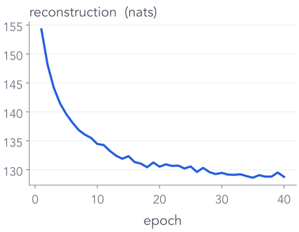
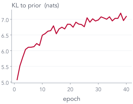
Reconstruction falls, KL rises, then both settle
After 40 epochs: reconstruction 128.8 + KL 7.1 = 135.9 nats per test image.
The payoff
Generate: random code → decoder. No encoder.
This is the whole generator. The encoder was scaffolding for training.
48 random codes each
Samples from two VAEs
2-number code · reconstruction 128.8
16-number code · reconstruction 57.8
More code dimensions: sharper and more varied, but some samples are odd. Neither is perfect.
Because the code is 2-D, we can draw the whole map
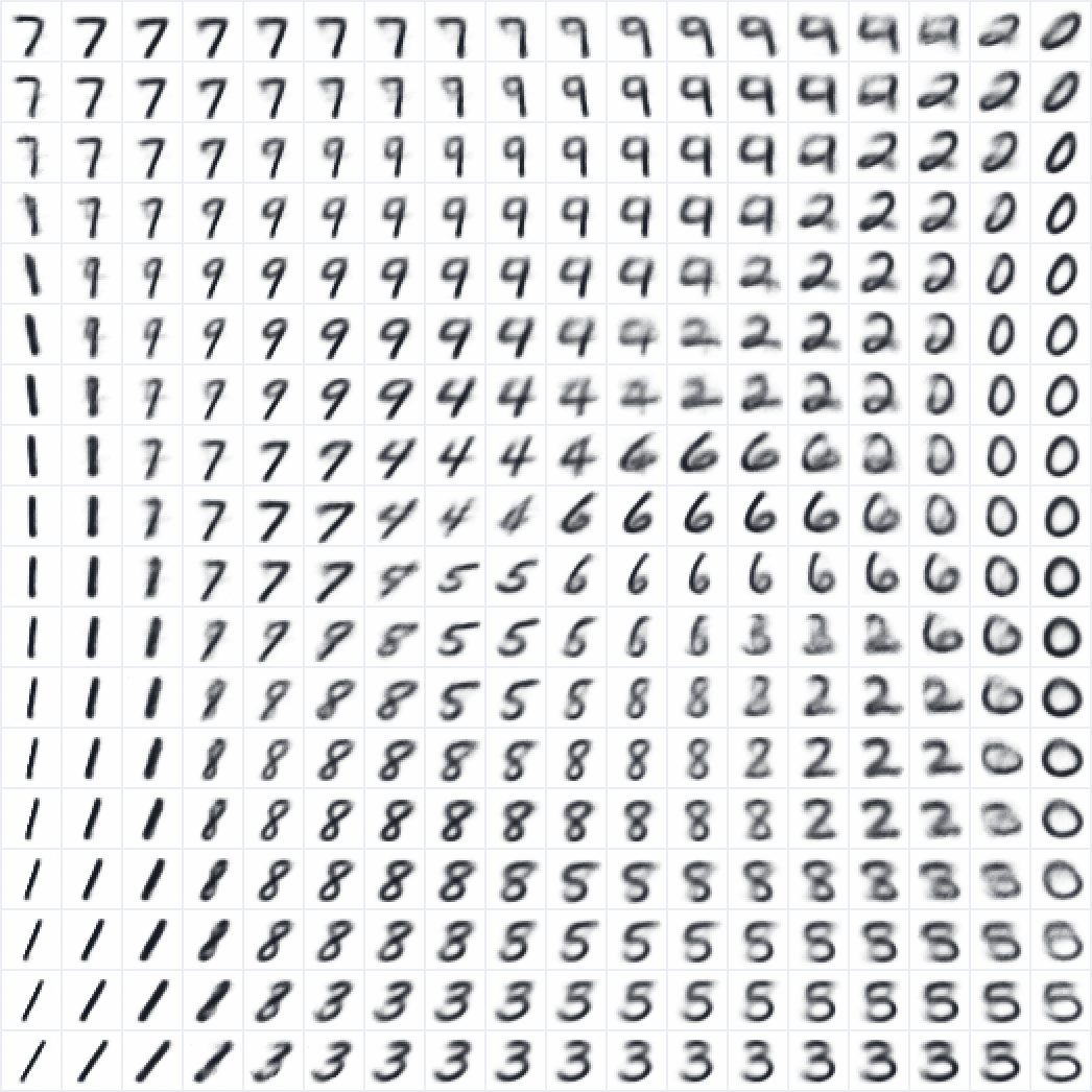
Every point in the code space is a digit
where test digits land
decoded on an 18 × 18 grid, spaced by quantiles of $\N(0,1)$
Neighbouring codes give similar digits, and every region decodes to something plausible.
Try it: the trained VAE, in your browser
The same app, now for the VAE
decoded from $z$the real digit
$z$ = (, )
Now random codes from $\N(0, I)$ land among the dots, and almost every one decodes to a digit.
The cover, explained
Walk in a straight line from our 3 to a 7
encode both, take 12 evenly spaced points between their $\mu$'s, decode each (16-number VAE)
the same walk in the 2-number VAE: the line passes through the 5, 8, 4 and 9 regions on the map
The tug of war, made visible
No KL, normal KL, too much KL
autoencoder (no KL)
recon 128.1 · no KL term
VAE, loss = recon + KL
recon 128.8 · KL 7.1
recon + 8 × KL
recon 140.4 · KL 3.9
Rows: code space · reconstructions · random samples. Too little KL: samples fail. Too much: everything blurs together.
An honest look
Why are VAE samples blurry?
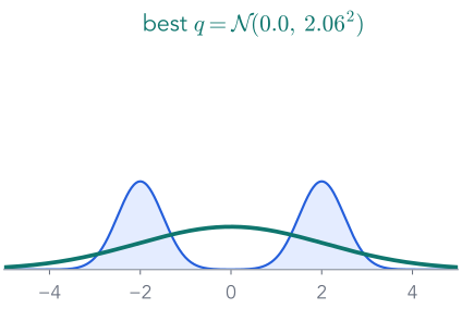
1. It fits $\KL(\text{data}\,\|\,\text{model})$. Like the wide Gaussian on our bumps, it must cover every training digit, so when unsure it spreads probability.
2. Pixels are independent given $z$. The decoder outputs one probability per pixel. If a stroke could be here or one pixel over, the best $\pi$ is grey in both places.
3. We show $\pi$, the mean, not a sample. A sample would be speckled instead of grey.
$\pi$ (the mean)
a sample
Not a law of nature: bigger codes, better decoders and better likelihoods all sharpen VAEs.
End of Part 7
What we did, and what comes next
What we did
Our 3: encode to a cloud, sample a code, decode, score: loss $= 129.3$.
Training: reconstruction falls, KL rises, both settle.
Generation needs only the prior and the decoder.
The KL weight trades sharp reconstructions against a usable code space; samples blur.
Next lecture: a different idea
VAEs maximise a bound on $p_\theta(x)$. GANs skip $p_\theta(x)$ entirely: a second network learns to judge real from fake.
Three ways to generate
Same goal, three different training signals
Return to the opening
What you can now explain
the cover: encode a 3 and a 7, walk a straight line between their codes, decode each point.
every code in $\N(0, I)$ decodes to a digit: recon + KL, derived from $\KL(q\,\|\,\text{posterior})$.
a conditional VAE: give the label to the encoder and the decoder, and choose which digit to draw.
Before you leave
Three exit questions
To generate a new digit with a trained VAE, which parts of the network do you use?
The prior and the decoder only: $z\sim\N(0, I)$, then decode. The encoder is for training.
Two different KL divergences appear in the VAE story. What does each compare, and which one is in the loss?
$\KL(q\,\|\,\text{prior})$ is in the loss (6.97 for our 3). $\KL(q\,\|\,\text{true posterior})$ is the gap between the ELBO and $\log p_\theta(x)$ (0.55).
We never compute $p_\theta(x)$. Why does maximising the ELBO still pull $q$ towards the true posterior?
$\log p_\theta(x) = \ELBO + \KL(q\,\|\,\text{posterior})$, and the left side does not depend on $q$. Whatever the ELBO gains, the KL loses.
After the GAN lecture
What if we generate by removing noise, a little at a time?
our 3
→ add a little Gaussian noise, again and again →
pure noise
Adding noise is easy and gives free training pairs. Can a network learn to undo one small step, then walk all the way back from pure noise?
Appendix
A second route to the ELBO
The VI lecture (its Part 6) reached the ELBO from $\KL(q\,\|\,\text{posterior})$. Many textbooks reach it from $\log p_\theta(x)$ with Jensen's inequality instead. Same bound, one more tool.
Multiplying and dividing by the same positive number changes nothing. We are free to choose any $q$; we choose the encoder's Gaussian, which is positive everywhere.
Why bother? Because the next move turns this integral into an average under $q$, and $q$ knows where the patch is.
An integral against $q$ is an average under $q$: $\int q(z)\,f(z)\,dz = \E_{z\sim q}[f(z)]$. Here $f(z)$ is the ratio $p_\theta(x,z)/q_\varphi(z\mid x)$: one number for each code.
Still exact. We now average over codes drawn from the encoder's cloud, right where the patch is.
Appendix · the ELBO through Jensen · a tool for move 4
Jensen's inequality, in one picture
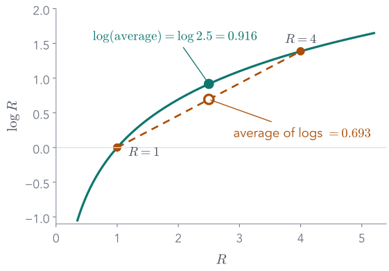
$\log$ curves downwards (it is concave), so every chord lies below the curve.
Two values, $R=1$ and $R=4$:
$$\underbrace{\log 2.5}_{\log \text{ of the average}} = 0.916 \;\ge\; \underbrace{\tfrac12(0 + 1.386)}_{\text{average of the logs}} = 0.693$$
Blei, Kucukelbir & McAuliffe, Variational Inference: A Review for Statisticians, arXiv 1601.00670
Bishop, Pattern Recognition and Machine Learning, §10.1: the ELBO + KL picture of Part 5
The VI lecture (vi.html): KL, the ELBO and reparameterisation on toys; and three YouTube videos on KL divergence (video ids sjgZxuCm_8Q, KHVR587oW8I, tXE23653JrU)
Stanford CS236 notes on VAEs (deepgenerativemodels.github.io)
This lecture's code: scripts/train_models.py (all models), scripts/make_figures.py and make_figures_extra.py (every number on the slides)












 →
 →
 →
 →

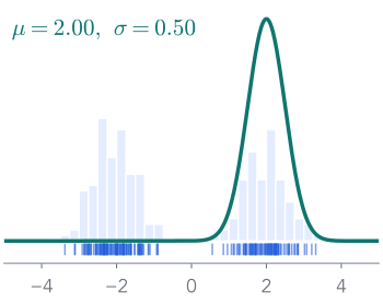 $\log p = −3746.0$
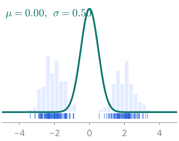 $\log p = −1790.0$
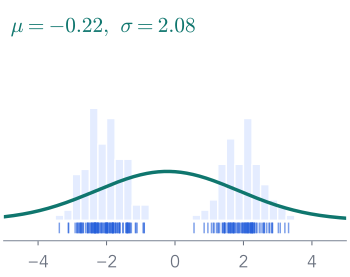 $\log p = −430.0$