Session 2 · KL, variational inference, the VAE

Session 2 · where we stopped

Last time: we need $q$ close to a posterior we cannot compute

A decoder plus a prior is a probability model: $p(z)\,p_\theta(x\mid z)$.

Training it needs $p_\theta(x) = \int p(z)\,p_\theta(x\mid z)\,dz$: intractable.

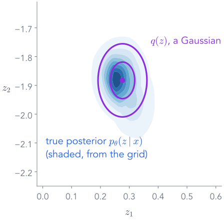
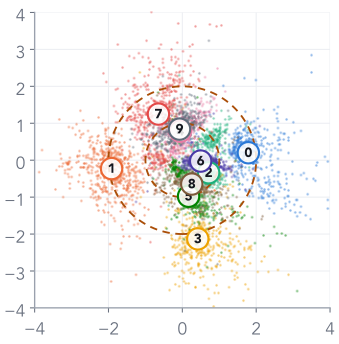
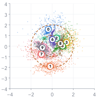
So does the posterior $p_\theta(z\mid x)$, the shaded patch for our 3.

Variational idea: a simple Gaussian $q$ (purple), pulled close to it.

The VI lecture's two lines:
$\log p(D) = \ELBO(q) + \KL\big(q\,\|\,p(\theta\mid D)\big)$ for every $q$
$z = \mu + \sigma\cdot\eps$: a random draw with a gradient

Today: those two lines for our 3, then one network that applies them to every image: the VAE.

Part 4 of 7

KL divergence, recalled for our 3's code

We want $q$ close to the posterior. The VI lecture built "close" from scratch (its Part 2). Here: the facts we need from it, and the one formula every VAE loss uses, a cloud against the prior $\N(0, I)$.

✓Distributions and fitting
✓Autoencoders
✓The probabilistic view
4KL divergence
5Variational inference and the ELBO
6Reparameterisation
7The VAE on MNIST

From the VI lecture, Part 2

KL is an average of log-ratios, under its first argument

$$\KL\big(q\,\|\,p\big) = \E_{z\sim q}\big[\log q(z) - \log p(z)\big]$$

Never negative

$\KL \ge 0$, and $= 0$ only when $q = p$: the log lies below its tangent.

Not symmetric

$\KL(q\|p) \ne \KL(p\|q)$. Which one we minimise changes the answer.

VI uses $\KL(q\,\|\,\text{posterior})$

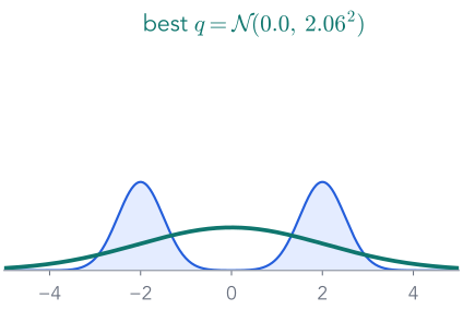
An average under $q$, which we can draw from. The price: $q$ seeks one mode and comes out too narrow.

Our 3's posterior is a single small patch, so there is only one mode to seek. What a diagonal $q$ cannot do is tilt with it.

VI lecture (vi.html), Part 2: KL for densities, never negative, not symmetric · KL between two Gaussians, live · forward vs reverse on two bumps

The KL in every VAE loss

A Gaussian cloud against the prior $\N(0, 1)$

The VI lecture's formula for two Gaussians:

$$\KL(q\,\|\,p) = \frac12\left[\log\frac{\sigma_p^2}{\sigma_q^2} - 1 + \frac{\sigma_q^2 + (\mu_q-\mu_p)^2}{\sigma_p^2}\right]$$

Put in the prior, $\mu_p = 0$ and $\sigma_p = 1$:

$$\KL\big(q\,\|\,\N(0,1)\big) = \hl{\tfrac12\big(\mu^2 + \sigma^2 - 1 - \log\sigma^2\big)}$$

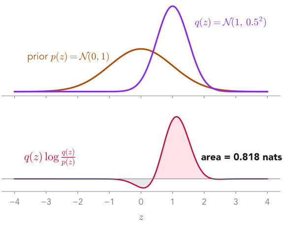
Check on the toy cloud $q = \N(1, 0.5^2)$, the shaded area:

$$\tfrac12\big(1 + 0.25 - 1 + 1.386\big) = 0.818\ \checkmark$$

A code with several coordinates and a diagonal $q$: one such term per coordinate, added. Moving a centre costs $\tfrac12\mu^2$; a width other than 1 costs $\tfrac12(\sigma^2 - 1 - \log\sigma^2)$.

VI lecture (vi.html), Part 2: derive the Gaussian KL · the answer, and torch's _kl_normal_normal

End of Part 4

What we did, and what comes next

What we did

From the VI lecture: $\KL(q\|p)$ is an average under $q$, never negative, not symmetric.
VI minimises $\KL(q\,\|\,\text{posterior})$ because we can draw from $q$; $q$ seeks a mode.
Against the prior: $\tfrac12(\mu^2+\sigma^2-1-\log\sigma^2)$ per coordinate, added.

Next: make $q$ close to the posterior

$\KL(q\,\|\,p_\theta(z\mid x))$ contains the intractable $p_\theta(x)$. The VI lecture's ELBO removes it; Part 5 runs it on our 3, then hands the job to an encoder.

Part 5 of 7

Variational inference for our 3, then for every image

The VI lecture turned "make $q$ close to the posterior" into a loss we can compute, the ELBO, and fitted a coin with it (its Part 6). Here the unknown is our 3's code: run the same loss on it, read the numbers, and see why doing this image by image leads to an encoder.

✓Distributions and fitting
✓Autoencoders
✓The probabilistic view
✓KL divergence
5Variational inference and the ELBO
6Reparameterisation
7The VAE on MNIST

From the VI lecture, Part 6, with an image in place of the coin

The same identity, written for one image

$$\log p_\theta(x) = \underbrace{\E_{z\sim q}\big[\log p_\theta(x, z) - \log q(z)\big]}_{\ELBO(q)} + \underbrace{\KL\big(q\,\|\,p_\theta(z\mid x)\big)}_{\ge\, 0}$$

VI lecture	here
$\theta$, the unknown	$z$, our 3's code
$D$, the data	$x$, our 3
prior $p(\theta)$	$p(z) = \N(0, I)$
likelihood $p(D\mid\theta)$	decoder $p_\theta(x\mid z)$

The ELBO needs only the joint, $p_\theta(x, z) = p(z)\,p_\theta(x\mid z)$: prior times decoder. No $p_\theta(x)$, no posterior.

$\log p_\theta(x)$ does not move when $q$ does, so whatever the ELBO gains, the KL to the posterior loses.

Careful with one letter: there, $\theta$ was the unknown; here it names the decoder's weights, and the unknown is $z$.

VI lecture (vi.html), Part 6: the catch · substitute Bayes · the evidence comes out · the lower bound · ELBO + KL for the coin

The lower bound, measured on our 3

The KL is never negative, so the ELBO sits below $\log p_\theta(x)$

$$\log p_\theta(x) = \ELBO(q) + \underbrace{\KL\big(q\,\|\,p_\theta(z\mid x)\big)}_{\ge\, 0} \;\ge\; \ELBO(q)$$

Our 3, two choices of $q$. The right end, $\log p_\theta(x)$, is fixed by the model; it does not move when $q$ changes.

$q = \N(0, I)$,
the prior

ELBO−386.2

$\log p_\theta(x)$−128.75

gap = KL to the posterior: about 257 nats

$q$ after variational
inference (next slides)

ELBO −128.83 · gap 0.08the two points overlap

The total cannot move, so raising the ELBO must shrink the KL: maximise the ELBO and $q$ approaches the posterior, without ever computing $p_\theta(x)$.

The VI lecture's second form, for an image

The ELBO, in symbols and in words

$$\ELBO = \E_{q}\big[\log p_\theta(x\mid z) + \log p(z) - \log q(z)\big]$$

$$\ELBO = \underbrace{\E_{z\sim\cenc q}\big[\cdec{\log p_\theta(x\mid z)}\big]}_{\text{rebuild } x \text{ from codes in its cloud}} \;-\; \underbrace{\closs{\KL\big(q(z)\,\|\,p(z)\big)}}_{\text{keep the cloud near } \N(0,I)}$$

First term: the autoencoder's reconstruction score, with the code drawn from the cloud.

Second term: the Gaussian KL to the prior from Part 4, in closed form.

The two wishes from the end of Part 2, derived rather than invented: rebuild well, and keep codes where the prior can find them.

VI lecture (vi.html), Part 6: two ways to write the same ELBO

Variational inference by hand, for our 3

Four numbers, gradient ascent on the ELBO

x = our_3                                  # 784 pixels, fixed
m     = torch.zeros(2, requires_grad=True)   # q's centre
log_s = torch.zeros(2, requires_grad=True)   # q's log-widths
opt = torch.optim.Adam([m, log_s], lr=0.03)

for step in range(800):
    z = m + log_s.exp() * torch.randn(64, 2)    # 64 draws from q
    rec = -bce(decoder(z), x).sum(1).mean()    # E_q[log p(x|z)]
    kl  = 0.5 * (m**2 + (2*log_s).exp() - 1 - 2*log_s).sum()
    loss = -(rec - kl)                           # minus the ELBO
    opt.zero_grad(); loss.backward(); opt.step()

Only $q$ is learned. The decoder is a trained one, kept fixed; $x$ is our 3. Start at $q = \N(0, I)$: $m = 0$, $s = 1$.

Draw codes from $q$: centre plus width times standard noise: the VI lecture's reparameterised draw (its Part 5), so gradients reach m and log_s.

The two terms: reconstruction, averaged over the 64 draws; the KL to the prior by the Gaussian formula from Part 4.

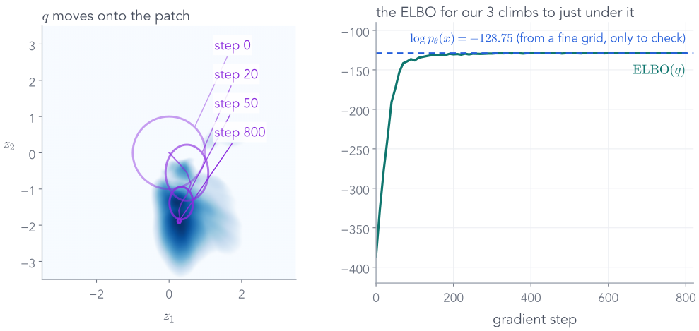
The same three-line loop as fitting one Gaussian in Part 1. The ELBO rises from −386.0 to −128.8.

Watch $q$ travel

From $\N(0, I)$ to our 3's patch in 800 steps

Final ELBO −128.83, just under $\log p_\theta(x) = −128.75$. The gap, $\KL(q\,\|\,\text{posterior})$, is 0.08 nats: $q$ is almost exactly right.

Inside those 800 steps

The two terms pull against each other

step	reconstruction $\E_q[\log p_\theta(x\mid z)]$	$-\,\KL(q\,\\|\,\text{prior})$	ELBO
0 · $q$ is the prior	−386.2	$-\,$0.0	−386.2
20	−275.9	$-\,$0.53	−276.4
50	−170.9	$-\,$2.1	−173.0
800	−122.2	$-\,$6.73	−128.9

Reconstruction gains about 264 nats: codes from $q$ now decode to our 3.

The KL to the prior grows from 0 to 6.73: a narrow cloud far from the origin costs something.

The ELBO is a trade: a $q$ precise enough to rebuild the image, no more precise than it needs to be.

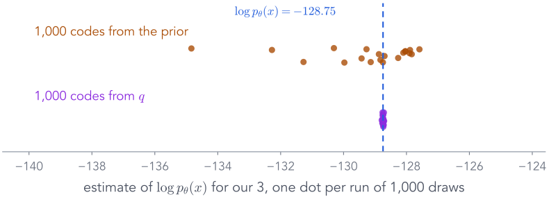
A bonus: with $q$, even $p_\theta(x)$ becomes easy to estimate

Sample codes where the patch is, then reweight

$$p_\theta(x) = \int q(z)\,\frac{p(z)\,p_\theta(x\mid z)}{q(z)}\,dz = \E_{z\sim q}\!\left[\frac{p_\theta(x, z)}{q(z)}\right] \approx \frac1S\sum_{s=1}^{S}\frac{p_\theta(x, z_s)}{q(z_s)}$$

20 runs of 1,000 draws each. From the prior, the estimates scatter from −134.8 to −127.6. From $q$: −128.74, give or take 0.017.

800 steps for one image

Amortised inference: learn to predict $q$

Our 3: ELBO −128.83 by hand in 800 steps, −129.3 from the encoder in one pass. Pay once during training; a little worse, thousands of times cheaper.

Put the pieces together

Encoder + decoder + ELBO = the variational autoencoder

$$\max_{\theta,\,\varphi}\;\sum_{i=1}^{N}\Big(\E_{z\sim\cenc{q_\varphi(z\mid x_i)}}\big[\cdec{\log p_\theta(x_i\mid z)}\big] - \closs{\KL\big(q_\varphi(z\mid x_i)\,\|\,p(z)\big)}\Big)$$

"Variational"

$q$ always depended on the image; now we write it $q_\varphi(z\mid x)$: the best Gaussian under the ELBO, predicted by a network.

"Autoencoder"

image → encoder → code → decoder → image: the shape from Part 2, now with a cloud for a code.

Trained together

Pushing on $\theta$ raises the ELBO mostly by making the data more probable: a better model. Pushing on $\varphi$ shrinks the gap: a better $q$.

Kingma & Welling (2014) and Rezende et al. (2014): one network for the likelihood, one for the posterior, one loss for both.

The gap for the encoder's $q$, measured on our 3

Two different KLs, two different jobs

ELBO−129.3

$\log p_\theta(x)$−128.75

gap $= \KL(q\,\|\,\text{true posterior}) = 0.55$

In the loss: $\KL(q\,\|\,\text{prior}) = 6.97$ nats. Computable by formula.

In the gap: $\KL(q\,\|\,\text{true posterior}) = 0.55$ nats. Needs $p_\theta(x)$; we only got it from the grid.

VI by hand closed the gap to 0.08 nats in 800 steps; the encoder's single pass leaves 0.55. That small loss is the price of amortising.

End of Part 5

What we did, and what comes next

What we did

Our 3: $\log p_\theta(x) = \ELBO + \KL(q\,\|\,\text{posterior})$, as in the VI lecture.
ELBO = reconstruction $-\ \KL(q\,\|\,\text{prior})$: both computable.
VI by hand fits our 3's $q$ in 800 steps and leaves a gap of 0.08 nats.
An encoder predicts $q$ in one pass, with a gap of 0.55: that is the VAE.

Next: gradients through a random draw

The loss draws $z$ from the encoder's cloud. Part 6: the VI lecture's reparameterisation, with $\mu$ and $\log\sigma^2$ coming out of a network.

Part 6 of 7

Backpropagating through the encoder's random draw

VI by hand drew each code as $m + s\cdot\eps$ and backpropagated through it: the VI lecture's reparameterisation trick (its Part 5). The VAE does the same, except that $\mu$ and $\sigma$ come out of the encoder, as $\log\sigma^2$. One recalled picture, one more link in the chain, and three lines of PyTorch.

✓Distributions and fitting
✓Autoencoders
✓The probabilistic view
✓KL divergence
✓Variational inference and the ELBO
6Reparameterisation
7The VAE on MNIST

From the VI lecture, Part 5, with the encoder in front

Draw $\eps$ first, and the path back to $\mu$ and $\sigma$ is arithmetic

As the VI lecture showed, sample() would cut the graph at $z$. Each draw gives a noisy gradient; on average it is exact.

VI lecture (vi.html), Part 5: the blocked graph · sample() fails · the reparameterised graph · checked in code · rsample

What the encoder adds: one more link in the chain

The encoder outputs $v = \log\sigma^2$, not $\sigma$

$\sigma$$=$$e^{v/2}$ $v$ can be any real number; $\sigma$ is always positive $\dfrac{\partial\sigma}{\partial v}$$=$$\tfrac12 e^{v/2} = \dfrac{\sigma}{2}$ derivative of $e^{v/2}$ $\dfrac{\partial z}{\partial v}$$=$$\dfrac{\partial z}{\partial\sigma}\cdot\dfrac{\partial\sigma}{\partial v} = \eps\cdot\dfrac{\sigma}{2}$ one more chain-rule factor after $\partial z/\partial\sigma = \eps$ $\dfrac{\partial z_1}{\partial v_1}$$=$$0.62 \times \dfrac{ 0.047 }{2} = 0.015$ our 3: $v_1 = −6.11$, so $\sigma_1 = 0.047$; this draw's $\eps_1 = 0.62$

Autograd adds this factor for us: in code it is the one line std = torch.exp(0.5 * logvar).

In PyTorch

Three lines

# encoder outputs, shape [B, 2] each
mu, logvar = encoder(x)
std = torch.exp(0.5 * logvar)     # sigma = exp(v / 2)
eps = torch.randn_like(std)       # standard normal, no grad
z   = mu + std * eps              # differentiable in mu, std

std is $\sigma = e^{v/2}$: the extra link from the last slide.

Normal(mu, std).rsample() does the same thing, as in the VI lecture; .sample() drops the gradient.

For our 3: $\mu = (0.3,\, −1.93)$, $\eps = (0.62,\, −1.15)$ gives $z = (0.33,\, −1.99)$.

End of Part 6

What we did, and what comes next

What we did

From the VI lecture: sampling $z$ directly cuts the gradient path; $z = \mu + \sigma\eps$ with $\eps \sim \N(0, I)$ keeps it.
$\partial z/\partial\mu = 1$ and $\partial z/\partial\sigma = \eps$; one draw is noisy, the average is exact.
The encoder outputs $v = \log\sigma^2$: one more factor, $\partial\sigma/\partial v = \sigma/2$.
In PyTorch: three lines, or rsample().

Next: everything together

Encoder, cloud, reparameterised sample, decoder, ELBO: train it on MNIST and follow our 3 through every step.

Part 7 of 7

The variational autoencoder, end to end

Every piece is in place: encoder, cloud, KL, ELBO, reparameterisation. Follow our 3 through the trained network, then generate.

✓Distributions and fitting
✓Autoencoders
✓The probabilistic view
✓KL divergence
✓Variational inference and the ELBO
✓Reparameterisation
7The VAE on MNIST

Our 3 through the trained VAE · 1 of 3

Encode: the image becomes a cloud

$\sigma \approx 0.05$ against the prior's $\sigma = 1$: the encoder is very sure where our 3 belongs.

Our 3 through the trained VAE · 2 of 3

Sample: one code from inside the cloud

Our 3 through the trained VAE · 3 of 3

Decode, then score against the real 3

Loss for our 3: $122.3 + 6.97 = 129.3$ nats. Backpropagate it into both $\theta$ and $\varphi$.

Step 3, zoomed in: the reconstruction term

Each pixel is a coin flip with probability $\pi_i$

our 3, one 5 × 5 patch

$$-\log p_\theta(x\mid z) = -\sum_{i=1}^{784}\Big[x_i\log\pi_i + (1-x_i)\log(1-\pi_i)\Big] = 122.3\ \text{nats}$$

Binary cross-entropy is not a design choice: it is the Bernoulli log-likelihood. Gaussian pixels would give squared error.

All three steps on one page

The whole VAE, for our 3

The same network as tensors

Shapes, layer by layer

The KL term for our 3

A tight cloud is expensive

$$\KL = \tfrac12\sum_{j}\big(\mu_j^2 + \sigma_j^2 - 1 - \log\sigma_j^2\big)$$

coordinate	$\mu_j$	$\sigma_j$	$\mu_j^2$	$\sigma_j^2 - 1$	$-\log\sigma_j^2$	$\tfrac12(\text{sum})$
$z_1$	0.3	0.047	0.09	$-1.00$	6.11	2.6
$z_2$	−1.93	0.05	3.72	$-1.00$	6.00	4.37
total						6.97 nats

$$-\log\sigma_1^2 = -\log(0.047^2) = -\log 0.0022 = 6.11$$

Most of the cost is $-\log\sigma^2$: the price of being precise. Reconstruction wants precision; the KL resists.

One training step

The whole algorithm fits on a slide

mu, logvar = model.encoder(x)              # [B,2], [B,2]
z = mu + torch.exp(0.5*logvar) * torch.randn_like(mu)
logits = model.decoder(z)                  # [B,784]
recon = F.binary_cross_entropy_with_logits(
          logits, x.flatten(1), reduction="none").sum(1)
kl = 0.5 * (mu**2 + logvar.exp() - 1 - logvar).sum(1)
loss = (recon + kl).mean()                 # per image, then batch
opt.zero_grad(); loss.backward(); opt.step()

Encode, reparameterise, decode.

Sum the BCE over all 784 pixels of each image.

Sum the KL over the 2 code coordinates of each image.

Add per image, average over the batch, step both encoder and decoder.

Averaging BCE over pixels instead of summing silently makes the KL 784× stronger.

Training run, test set

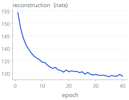
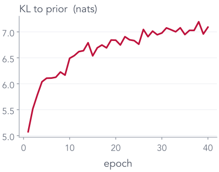
Reconstruction falls, KL rises, then both settle

After 40 epochs: reconstruction 128.8 + KL 7.1 = 135.9 nats per test image.

The payoff

Generate: random code → decoder. No encoder.

This is the whole generator. The encoder was scaffolding for training.

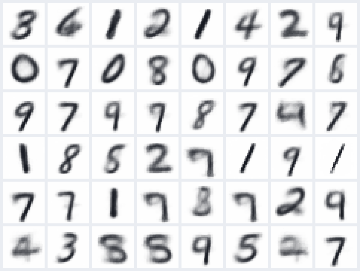
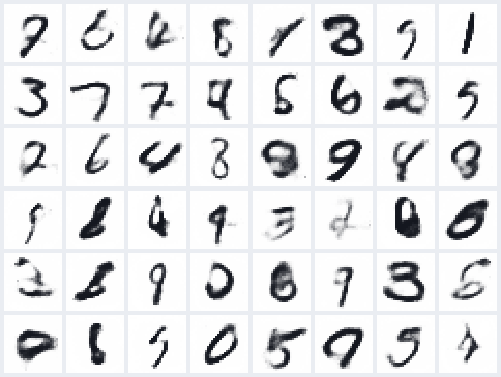
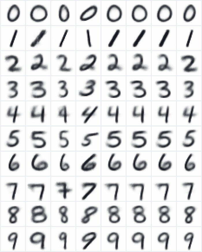
48 random codes each

Samples from two VAEs

2-number code · reconstruction 128.8

16-number code · reconstruction 57.8

More code dimensions: sharper and more varied, but some samples are odd. Neither is perfect.

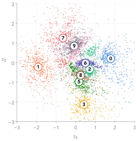
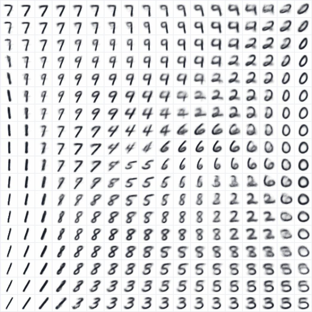
Because the code is 2-D, we can draw the whole map

Every point in the code space is a digit

where test digits land

decoded on an 18 × 18 grid, spaced by quantiles of $\N(0,1)$

Neighbouring codes give similar digits, and every region decodes to something plausible.

Try it: the trained VAE, in your browser

The same app, now for the VAE

decoded from $z$

the real digit

$z$ = (, )

$z_1$ $z_2$

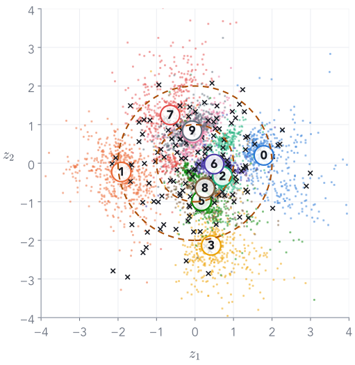
Now random codes from $\N(0, I)$ land among the dots, and almost every one decodes to a digit.

The cover, explained

Walk in a straight line from our 3 to a 7

encode both, take 12 evenly spaced points between their $\mu$'s, decode each (16-number VAE)

the same walk in the 2-number VAE: the line passes through the 5, 8, 4 and 9 regions on the map

The tug of war, made visible

No KL, normal KL, too much KL

autoencoder (no KL)

recon 128.1 · no KL term

VAE, loss = recon + KL

recon 128.8 · KL 7.1

recon + 8 × KL

recon 140.4 · KL 3.9

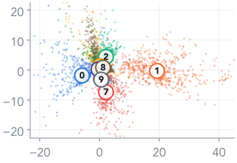
Rows: code space · reconstructions · random samples. Too little KL: samples fail. Too much: everything blurs together.

An honest look

Why are VAE samples blurry?

1. It fits $\KL(\text{data}\,\|\,\text{model})$. Like the wide Gaussian on our bumps, it must cover every training digit, so when unsure it spreads probability.

2. Pixels are independent given $z$. The decoder outputs one probability per pixel. If a stroke could be here or one pixel over, the best $\pi$ is grey in both places.

3. We show $\pi$, the mean, not a sample. A sample would be speckled instead of grey.

$\pi$ (the mean)

a sample

Not a law of nature: bigger codes, better decoders and better likelihoods all sharpen VAEs.

End of Part 7

What we did, and what comes next

What we did

Our 3: encode to a cloud, sample a code, decode, score: loss $= 129.3$.
Training: reconstruction falls, KL rises, both settle.
Generation needs only the prior and the decoder.
The KL weight trades sharp reconstructions against a usable code space; samples blur.

Next lecture: a different idea

VAEs maximise a bound on $p_\theta(x)$. GANs skip $p_\theta(x)$ entirely: a second network learns to judge real from fake.

Three ways to generate

Same goal, three different training signals

Return to the opening

What you can now explain

the cover: encode a 3 and a 7, walk a straight line between their codes, decode each point.

every code in $\N(0, I)$ decodes to a digit: recon + KL, derived from $\KL(q\,\|\,\text{posterior})$.

a conditional VAE: give the label to the encoder and the decoder, and choose which digit to draw.

Before you leave

Three exit questions

To generate a new digit with a trained VAE, which parts of the network do you use? The prior and the decoder only: $z\sim\N(0, I)$, then decode. The encoder is for training.
Two different KL divergences appear in the VAE story. What does each compare, and which one is in the loss? $\KL(q\,\|\,\text{prior})$ is in the loss (6.97 for our 3). $\KL(q\,\|\,\text{true posterior})$ is the gap between the ELBO and $\log p_\theta(x)$ (0.55).
We never compute $p_\theta(x)$. Why does maximising the ELBO still pull $q$ towards the true posterior? $\log p_\theta(x) = \ELBO + \KL(q\,\|\,\text{posterior})$, and the left side does not depend on $q$. Whatever the ELBO gains, the KL loses.

After the GAN lecture

What if we generate by removing noise, a little at a time?

our 3

→ add a little Gaussian noise, again and again →

pure noise

Adding noise is easy and gives free training pairs. Can a network learn to undo one small step, then walk all the way back from pure noise?

Appendix

A second route to the ELBO

The VI lecture (its Part 6) reached the ELBO from $\KL(q\,\|\,\text{posterior})$. Many textbooks reach it from $\log p_\theta(x)$ with Jensen's inequality instead. Same bound, one more tool.

Appendix · the ELBO through Jensen · move 1 of 4

Start from what we want

$$\log p_\theta(x) = \log \int p_\theta(x,z)\,dz$$

Maximum likelihood wants this number large for our 3, and for every image in the data. The integral over all codes is the part we cannot compute.

A second route to the bound of Part 5, starting from $\log p_\theta(x)$ instead of the KL.

Appendix · the ELBO through Jensen · move 2 of 4

Multiply and divide by the encoder's cloud

$$\log \int p_\theta(x,z)\,dz$$

$$= \log \int \hl{q_\varphi(z\mid x)}\;\frac{p_\theta(x,z)}{\hl{q_\varphi(z\mid x)}}\,dz$$

Multiplying and dividing by the same positive number changes nothing. We are free to choose any $q$; we choose the encoder's Gaussian, which is positive everywhere.

Why bother? Because the next move turns this integral into an average under $q$, and $q$ knows where the patch is.

Appendix · the ELBO through Jensen · move 3 of 4

Read the integral as an average under $q$

$$\log \int q_\varphi(z\mid x)\,\frac{p_\theta(x,z)}{q_\varphi(z\mid x)}\,dz$$

$$= \log\; \hl{\E_{z\sim q_\varphi(z\mid x)}}\!\left[\frac{p_\theta(x,z)}{q_\varphi(z\mid x)}\right]$$

An integral against $q$ is an average under $q$: $\int q(z)\,f(z)\,dz = \E_{z\sim q}[f(z)]$. Here $f(z)$ is the ratio $p_\theta(x,z)/q_\varphi(z\mid x)$: one number for each code.

Still exact. We now average over codes drawn from the encoder's cloud, right where the patch is.

Appendix · the ELBO through Jensen · a tool for move 4

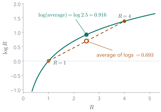
Jensen's inequality, in one picture

$\log$ curves downwards (it is concave), so every chord lies below the curve.

Two values, $R=1$ and $R=4$:

$$\underbrace{\log 2.5}_{\log \text{ of the average}} = 0.916 \;\ge\; \underbrace{\tfrac12(0 + 1.386)}_{\text{average of the logs}} = 0.693$$

$$\log \E[R] \;\ge\; \E[\log R]$$

Appendix · the ELBO through Jensen · move 4 of 4

Swap the log and the average: the only inequality

$$\log p_\theta(x) = \log\,\E_{q}\!\left[\frac{p_\theta(x,z)}{q_\varphi(z\mid x)}\right]$$

$$\log p_\theta(x) \;\hl{\ge}\; \E_{q}\!\left[\log\frac{p_\theta(x,z)}{q_\varphi(z\mid x)}\right] \;=:\; \ELBO$$

Jensen with $R = p_\theta(x,z)/q_\varphi(z\mid x)$. The right side is the Evidence Lower BOund: it can never exceed $\log p_\theta(x)$.

The same ELBO as Part 5. This route shows it is a bound; the KL route (the VI lecture's Part 6) also shows the gap is $\KL(q\,\|\,\text{posterior})$.

Where to go next

Lilian Weng, From Autoencoder to Beta-VAE (lilianweng.github.io): the autoencoder family of Part 2
Jaan Altosaar, Tutorial: what is a variational autoencoder?: the neural-network and probability views side by side
Kingma & Welling, Auto-Encoding Variational Bayes, arXiv 1312.6114
Blei, Kucukelbir & McAuliffe, Variational Inference: A Review for Statisticians, arXiv 1601.00670
Bishop, Pattern Recognition and Machine Learning, §10.1: the ELBO + KL picture of Part 5
The VI lecture (vi.html): KL, the ELBO and reparameterisation on toys; and three YouTube videos on KL divergence (video ids sjgZxuCm_8Q, KHVR587oW8I, tXE23653JrU)
Stanford CS236 notes on VAEs (deepgenerativemodels.github.io)
This lecture's code: scripts/train_models.py (all models), scripts/make_figures.py and make_figures_extra.py (every number on the slides)