In this first part, we’ll build a character-level language model from scratch. Given a sequence of characters, our model will learn to predict the next character. By doing this repeatedly, we can generate new text—in our case, new names.
This is the foundation of how large language models work, just at a much smaller scale.
The Big Picture
Input: "nipu" → Model → Output: probability distribution over next character
                                 'n': 0.7, 'a': 0.1, 'r': 0.05, ...
The model learns:
After “nipu”, ‘n’ is likely (forming “nipun”)
Names often end with ‘a’, ‘i’, or consonants
Certain character combinations are common in names
Setup
import torchimport torch.nn.functional as Ffrom torch import nnimport pandas as pdimport matplotlib.pyplot as pltimport osimport requests# Reproducibilitytorch.manual_seed(42)# Use GPU if availabledevice = torch.device("cuda"if torch.cuda.is_available() else"cpu")print(f"Using device: {device}")print(f"PyTorch version: {torch.__version__}")%config InlineBackend.figure_format ='retina'
Using device: cuda
PyTorch version: 2.6.0+cu124
Step 1: Get the Data
We’ll use a dataset of Indian names. Let’s download and explore it.
# Download the dataset if neededifnot os.path.exists('names.csv'):print("Downloading names dataset...") url ="https://raw.githubusercontent.com/balasahebgulave/Dataset-Indian-Names/master/Indian_Names.csv" response = requests.get(url)withopen('names.csv', 'w') as f: f.write(response.text)print("Download complete!")# Load and clean the datawords = pd.read_csv('names.csv')["Name"]words = words.str.lower().str.strip().str.replace(" ", "")words = words[words.str.len().between(3, 9)] # Keep reasonable length nameswords = words[words.apply(lambda x: x.isalpha())] # Only alphabeticwords = words.sample(frac=1, random_state=42).reset_index(drop=True) # Shufflewords = words.tolist()print(f"Total names: {len(words)}")print(f"Sample names: {words[:10]}")
# Create mappings# stoi: string to integer (character → number)# itos: integer to string (number → character)stoi = {ch: i +1for i, ch inenumerate(chars)}stoi['.'] =0# Special token for start/end of nameitos = {i: ch for ch, i in stoi.items()}vocab_size =len(stoi)print(f"Vocabulary size (including '.'): {vocab_size}")print(f"\nCharacter to index mapping:")print(stoi)
Start of name: The model sees “…..” and must predict the first character
End of name: The model predicts ‘.’ when the name is complete
This is similar to how LLMs use <BOS> (beginning of sequence) and <EOS> (end of sequence) tokens.
Step 3: Create Training Data
We need (input, target) pairs. For a name like “raj”:
Context (input)
Target
.....
r
....r
a
...ra
j
..raj
.
block_size =5# How many characters of context to usedef build_dataset(words, stoi, block_size):""" Convert words into training examples. For each word, slide a window of `block_size` characters and predict the next character. """ X, Y = [], []for word in words:# Start with a context of all '.' (zeros) context = [0] * block_sizefor ch in word +'.': # Include '.' to mark end target = stoi[ch] X.append(context.copy()) Y.append(target)# Slide window: remove first, add current character context = context[1:] + [target]return torch.tensor(X), torch.tensor(Y)X, Y = build_dataset(words, stoi, block_size)print(f"Dataset size: {len(X)} examples")print(f"Input shape: {X.shape}") # (num_examples, block_size)print(f"Target shape: {Y.shape}") # (num_examples,)
# Let's visualize a few examplesprint("First 10 training examples:")print("-"*40)for i inrange(10): context =''.join(itos[idx.item()] for idx in X[i]) target = itos[Y[i].item()]print(f"'{context}' → '{target}'")
We can’t feed characters directly to a neural network. Instead, we represent each character as a vector of numbers called an embedding.
# Each character becomes a vector of `emb_dim` numbersemb_dim =8# PyTorch's Embedding layer is just a lookup tableembedding = nn.Embedding(vocab_size, emb_dim)print(f"Embedding table shape: {embedding.weight.shape}")print(f" - {vocab_size} characters")print(f" - {emb_dim} dimensions each")
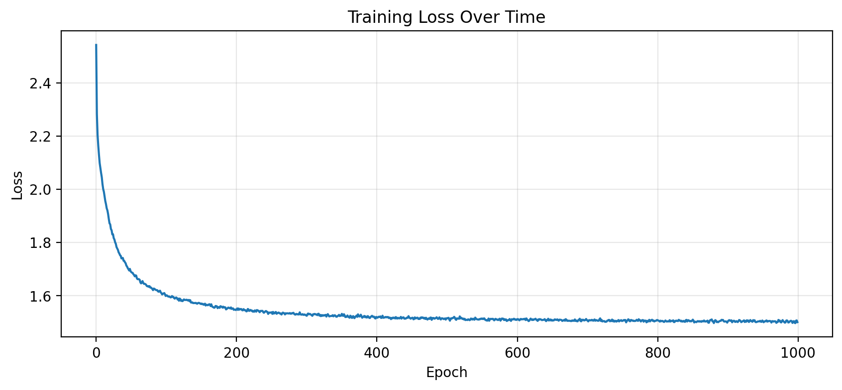
# Plot training lossplt.figure(figsize=(10, 4))plt.plot(losses)plt.xlabel('Epoch')plt.ylabel('Loss')plt.title('Training Loss Over Time')plt.grid(True, alpha=0.3)plt.show()
What does the loss mean?
Cross-entropy loss of ~2.0 means the model is, on average, as uncertain as if it were choosing between ~7 equally likely characters (since \(e^{2.0} \approx 7.4\)).
A random model would have loss \(\ln(27) \approx 3.3\) (uniform over 27 characters).
Step 7: Generate Names!
Now the fun part—let’s generate new names:
@torch.no_grad()def generate(model, itos, stoi, block_size, max_len=15, temperature=1.0):""" Generate a name character by character. Args: temperature: Controls randomness (lower = more deterministic) """ model.eval() context = [0] * block_size # Start with '.....' name = []for _ inrange(max_len):# Get model prediction x = torch.tensor([context]).to(device) logits = model(x)# Apply temperature probs = F.softmax(logits / temperature, dim=-1)# Sample from the distribution next_idx = torch.multinomial(probs, 1).item()# Check for end tokenif next_idx ==0:break name.append(itos[next_idx]) context = context[1:] + [next_idx]return''.join(name)
print("Generated Names:")print("="*40)for i inrange(20): name = generate(model, itos, stoi, block_size, temperature=0.8)print(f"{i+1:2d}. {name}")
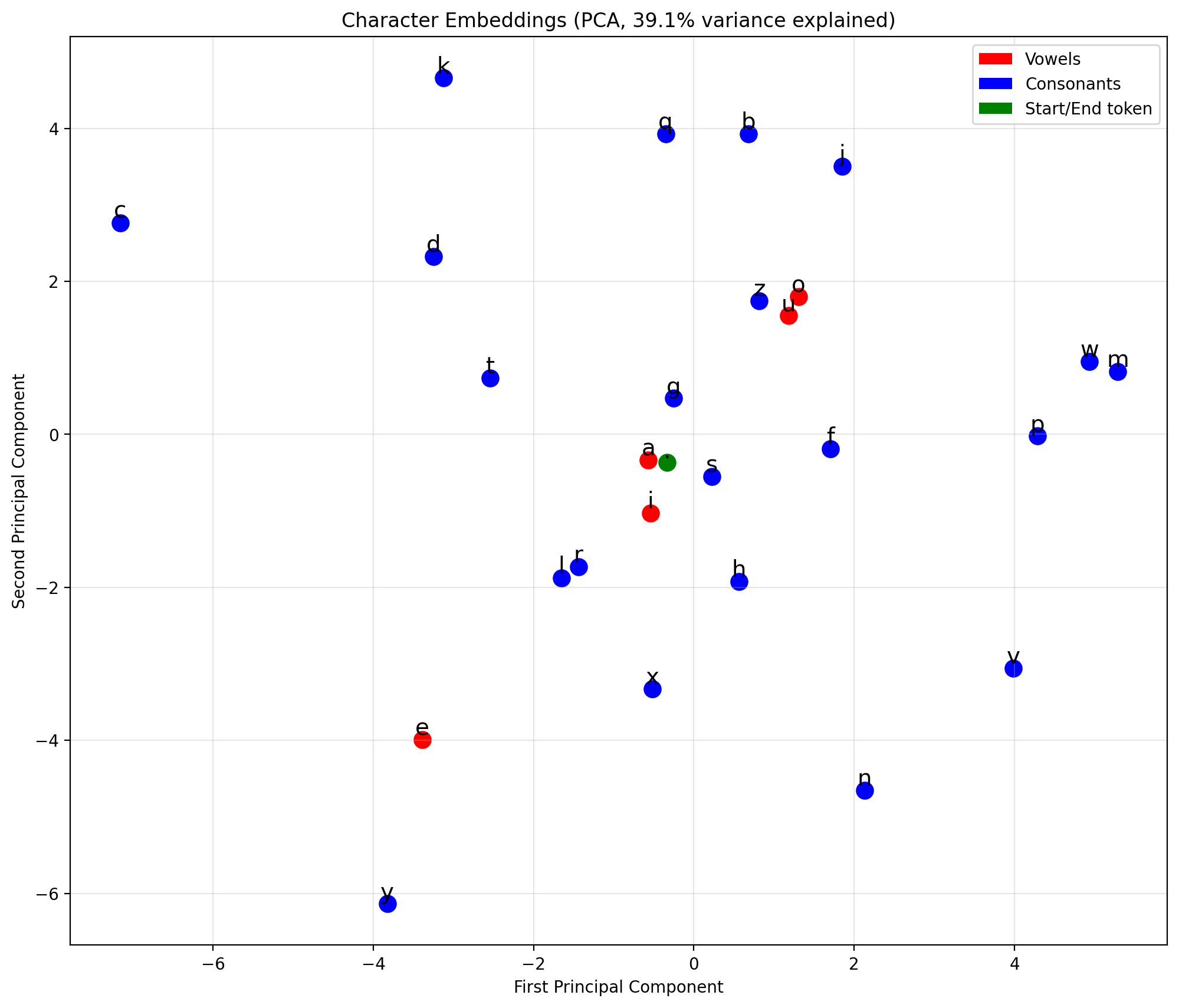
Let’s see how the model represents characters in embedding space:
from sklearn.decomposition import PCAdef plot_embeddings(model, itos):"""Visualize character embeddings using PCA.""" weights = model.emb.weight.detach().cpu().numpy()# Reduce to 2D for visualizationif weights.shape[1] >2: pca = PCA(n_components=2) weights_2d = pca.fit_transform(weights) explained =sum(pca.explained_variance_ratio_)else: weights_2d = weights explained =1.0 plt.figure(figsize=(12, 10))# Color code: vowels in red, consonants in blue vowels =set('aeiou')for i, (x, y) inenumerate(weights_2d): char = itos[i] color ='red'if char in vowels else ('green'if char =='.'else'blue') plt.scatter(x, y, c=color, s=100) plt.annotate(char, (x, y), fontsize=14, ha='center', va='bottom') plt.title(f'Character Embeddings (PCA, {explained:.1%} variance explained)') plt.xlabel('First Principal Component') plt.ylabel('Second Principal Component') plt.grid(True, alpha=0.3)# Legendfrom matplotlib.patches import Patch legend_elements = [ Patch(facecolor='red', label='Vowels'), Patch(facecolor='blue', label='Consonants'), Patch(facecolor='green', label='Start/End token') ] plt.legend(handles=legend_elements, loc='upper right') plt.show()plot_embeddings(model, itos)
What to look for
Vowels (a, e, i, o, u) often cluster together
Similar consonants may be near each other
The ‘.’ token (start/end) is usually separate
The model learned these relationships from data alone!
Save Model for Later Use
Let’s export the trained model and vocabulary so we can load it later for inference, comparison, or use in an app.
import pickle# Create models directoryos.makedirs('../models', exist_ok=True)# Save model checkpointcheckpoint = {'model_state_dict': model.state_dict(),'vocab_size': vocab_size,'block_size': block_size,'emb_dim': emb_dim,'hidden_size': hidden_size,'stoi': stoi,'itos': itos,}torch.save(checkpoint, '../models/char_lm_names.pt')print(f"Model saved to ../models/char_lm_names.pt")# Verify we can load itloaded = torch.load('../models/char_lm_names.pt', weights_only=False)print(f"Checkpoint keys: {list(loaded.keys())}")print(f"Model parameters: {sum(p.numel() for p in model.parameters()):,}")
Model saved to ../models/char_lm_names.pt
Checkpoint keys: ['model_state_dict', 'vocab_size', 'block_size', 'emb_dim', 'hidden_size', 'stoi', 'itos']
Model parameters: 17,651
Clean Up GPU Memory
When running multiple notebooks or experiments, it’s important to release GPU memory.
# Clean up GPU memoryimport gc# Delete model and data tensorsdel modeldel X, Y# Clear CUDA cacheif torch.cuda.is_available(): torch.cuda.empty_cache() torch.cuda.synchronize()# Run garbage collectiongc.collect()print("GPU memory cleared!")if torch.cuda.is_available():print(f"GPU memory allocated: {torch.cuda.memory_allocated() /1024**2:.1f} MB")print(f"GPU memory cached: {torch.cuda.memory_reserved() /1024**2:.1f} MB")
In this part, we built a complete character-level language model:
Component
Purpose
Vocabulary
Map characters ↔︎ integers
Embeddings
Represent characters as learnable vectors
Hidden layer
Learn patterns from context
Output layer
Predict next character distribution
Training loop
Learn from data via backpropagation
Generation
Sample from learned distribution
Key parameters:
block_size = 5: Characters of context
emb_dim = 8: Embedding dimensions
hidden_size = 128: Hidden layer size
Total: ~5,000 parameters
What’s Next
In Part 2, we’ll take this same architecture and train it on Shakespeare text. Same model, different data—showing that language models are general-purpose pattern learners.
Exercises
Experiment with block_size: What happens with 3 vs 8 characters of context?
Vary hidden_size: How does model capacity affect quality?
Temperature sampling: Try temperature 0.5 vs 1.5. What changes?
Add dropout: Implement regularization to prevent overfitting
Deeper networks: Add a second hidden layer. Does it help?