Mathematical Expectation and Law of Large Numbers
expectation, law of large numbers, running average, monte carlo simulation, dice simulation, bernoulli distribution, variance
Setting Up the Environment
We’ll use PyTorch for probability distributions, NumPy for numerical computations, Pandas for data manipulation, and Matplotlib for visualizations.
Dice Rolling Simulation: Understanding Expected Value
Let’s start with a classic example - rolling a fair six-sided die. The theoretical expected value of a fair die is:
\[E[X] = \frac{1 + 2 + 3 + 4 + 5 + 6}{6} = \frac{21}{6} = 3.5\]
Even though we can never actually roll a 3.5, this is the average value we expect over many rolls.
Observing Individual Dice Rolls
Let’s examine the frequency distribution of our dice rolls to see how they compare to the theoretical uniform distribution:
Computing Running Averages
Now let’s compute the running average to see how it converges to the theoretical expectation of 3.5:
The red dashed line shows the theoretical expected value of 3.5. Notice how the running average oscillates around this value and gradually converges to it as the number of rolls increases. This is a visual demonstration of the Law of Large Numbers.
Bernoulli Distribution and Expected Value
Let’s explore the Bernoulli distribution, which models binary outcomes (success/failure, heads/tails, etc.). For a Bernoulli random variable with probability \(p\) of success:
\[E[X] = 1 \cdot p + 0 \cdot (1-p) = p\]
So for a fair coin (\(p = 0.5\)), the expected value is 0.5.

Financial Application: Coin Flip Game
Now let’s explore a more complex application - a financial game based on coin flips. This demonstrates how expectation and variance work together in risk assessment.
Game Setup
In this game: - Each player plays 100 coin flips - Win ₹2000 for each heads - Lose ₹2000 for each tails - We simulate millions of players to understand the distribution of outcomes
plt.plot(runing_avg, lw=1)
plt.xlabel('Roll number')
plt.ylabel('Running average')
plt.axhline(3.5, color='red', lw=1, ls='--')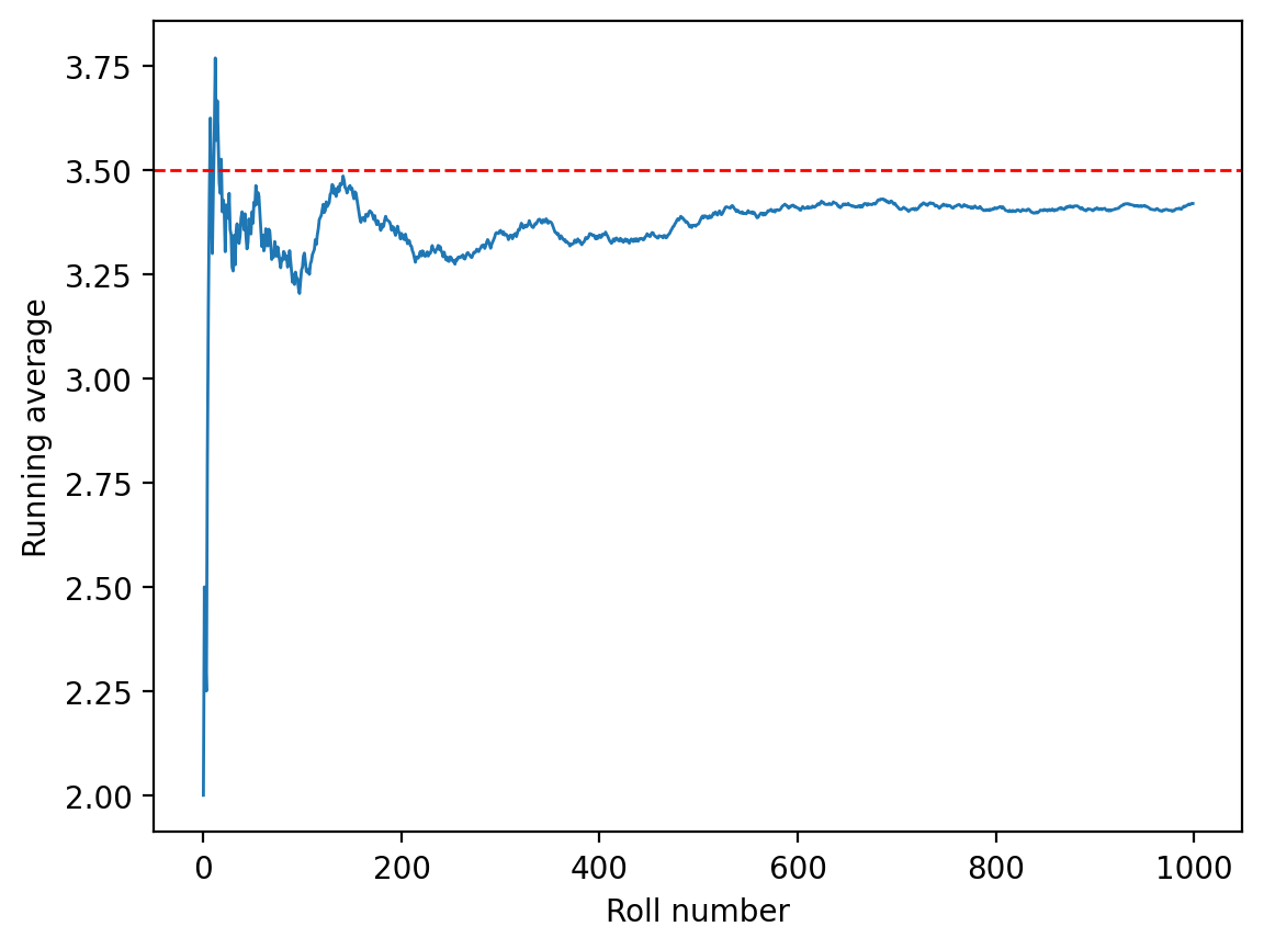
Distribution of Winnings
Let’s visualize the distribution of net money won across all players:
Expected Value and Variance Analysis
Let’s analyze the statistical properties of our game:
The ratio close to 1 confirms that our simulation matches the theoretical variance formula for the sum of independent random variables.
Alternative Simulation Approach: Individual Coin Flips
Let’s implement the same game using individual Bernoulli trials instead of the Binomial distribution to verify our results:
tensor([46., 54., 58., 58., 58., 55., 55., 47., 50., 54., 54., 40., 52., 54.,
        54., 44., 49., 53., 59., 43., 54., 47., 53., 46., 45., 55., 50., 48.,
        51., 56., 49., 42., 50., 52., 48., 53., 58., 47., 46., 46., 58., 60.,
        40., 44., 53., 47., 50., 52., 42., 50., 45., 52., 52., 51., 46., 33.,
        53., 52., 49., 42., 52., 44., 56., 49., 51., 55., 50., 53., 57., 50.,
        49., 53., 56., 53., 49., 48., 55., 50., 50., 48., 59., 53., 54., 37.,
        48., 57., 41., 60., 55., 59., 53., 55., 50., 46., 51., 47., 51., 44.,
43., 55.])0 -16000.0
1 16000.0
2 32000.0
3 32000.0
4 32000.0
...
4999995 -16000.0
4999996 52000.0
4999997 -44000.0
4999998 -4000.0
4999999 -20000.0
Length: 5000000, dtype: float32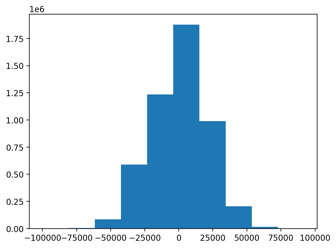
Visualizing Individual Player Trajectories
Let’s examine how individual players’ fortunes evolve over the course of their 100 coin flips:
This powerful visualization shows all player trajectories in gray (left) and the final distribution of outcomes (right). Notice how most trajectories cluster around zero net winnings, consistent with the fair game’s expected value of zero.
Mathematical Properties: Variance and Its Maximum
Let’s explore an important mathematical property - when does the variance of a Bernoulli distribution reach its maximum?
Verifying Expected Value of Binomial Distribution
Let’s verify that our simulation correctly captures the expected value of a Binomial distribution:
Advanced Example: Expectation of Gaussian Distribution
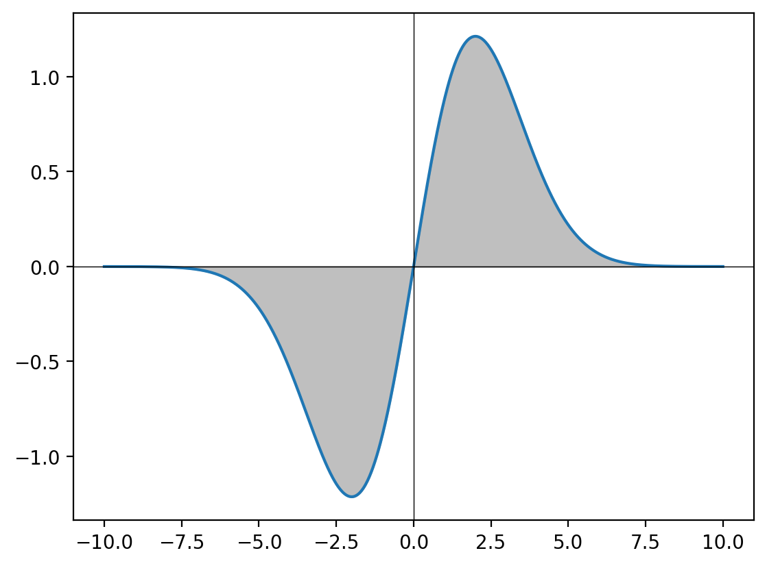
Let’s conclude with a more advanced example - computing the expected value of a Gaussian distribution using integration. For a standard normal distribution \(X \sim \mathcal{N}(0, \sigma^2)\):
\[E[X] = \int_{-\infty}^{\infty} x \cdot \frac{1}{\sqrt{2\pi\sigma^2}} e^{-\frac{x^2}{2\sigma^2}} dx = 0\]
This integral evaluates to zero because the function is odd and symmetric around zero.
Summary
In this notebook, we’ve explored the fundamental concept of mathematical expectation through:
- Theoretical Foundation: Understanding expected value as the long-run average
- Law of Large Numbers: Observing convergence through simulation
- Practical Applications: Financial modeling and risk assessment
- Statistical Properties: Variance and its relationship to expectation
- Advanced Concepts: Integration for continuous distributions
Key Takeaways
- Expected value provides the central tendency of a random variable
- The Law of Large Numbers guarantees convergence of sample means
- Variance measures the spread around the expected value
- Even fair games (zero expected value) can have high variance and risk
- Simulation is a powerful tool for understanding theoretical concepts
Next Steps
- Explore conditional expectation and its applications
- Study the Central Limit Theorem and its relationship to the Law of Large Numbers
- Investigate more complex probability distributions and their moments
- Apply these concepts to real-world data analysis problems
| 0 | 1 | 2 | 3 | 4 | 5 | 6 | 7 | 8 | 9 | ... | 90 | 91 | 92 | 93 | 94 | 95 | 96 | 97 | 98 | 99 | |
|---|---|---|---|---|---|---|---|---|---|---|---|---|---|---|---|---|---|---|---|---|---|
| 0 | 0.0 | 0.0 | 1.0 | 0.0 | 1.0 | 1.0 | 1.0 | 1.0 | 1.0 | 0.0 | ... | 1.0 | 0.0 | 1.0 | 1.0 | 1.0 | 1.0 | 1.0 | 0.0 | 0.0 | 1.0 |
| 1 | 0.0 | 0.0 | 0.0 | 1.0 | 1.0 | 0.0 | 1.0 | 0.0 | 0.0 | 1.0 | ... | 0.0 | 1.0 | 1.0 | 0.0 | 0.0 | 1.0 | 0.0 | 1.0 | 0.0 | 1.0 |
| 2 | 0.0 | 1.0 | 1.0 | 1.0 | 1.0 | 1.0 | 0.0 | 0.0 | 1.0 | 1.0 | ... | 1.0 | 1.0 | 0.0 | 1.0 | 1.0 | 1.0 | 1.0 | 0.0 | 1.0 | 1.0 |
| 3 | 1.0 | 1.0 | 1.0 | 0.0 | 0.0 | 0.0 | 1.0 | 1.0 | 0.0 | 0.0 | ... | 0.0 | 0.0 | 0.0 | 1.0 | 1.0 | 0.0 | 1.0 | 1.0 | 1.0 | 0.0 |
| 4 | 0.0 | 1.0 | 0.0 | 0.0 | 0.0 | 1.0 | 1.0 | 0.0 | 0.0 | 1.0 | ... | 1.0 | 0.0 | 1.0 | 0.0 | 1.0 | 1.0 | 1.0 | 0.0 | 1.0 | 1.0 |
5 rows × 100 columns
# win and loss -- replace 0 with -2000 and 1 with 2000
win_amount_df = overall_samples_df.replace({0: loss_amt, 1: win_amt})
win_amount_df.head()| 0 | 1 | 2 | 3 | 4 | 5 | 6 | 7 | 8 | 9 | ... | 90 | 91 | 92 | 93 | 94 | 95 | 96 | 97 | 98 | 99 | |
|---|---|---|---|---|---|---|---|---|---|---|---|---|---|---|---|---|---|---|---|---|---|
| 0 | -2000.0 | -2000.0 | 2000.0 | -2000.0 | 2000.0 | 2000.0 | 2000.0 | 2000.0 | 2000.0 | -2000.0 | ... | 2000.0 | -2000.0 | 2000.0 | 2000.0 | 2000.0 | 2000.0 | 2000.0 | -2000.0 | -2000.0 | 2000.0 |
| 1 | -2000.0 | -2000.0 | -2000.0 | 2000.0 | 2000.0 | -2000.0 | 2000.0 | -2000.0 | -2000.0 | 2000.0 | ... | -2000.0 | 2000.0 | 2000.0 | -2000.0 | -2000.0 | 2000.0 | -2000.0 | 2000.0 | -2000.0 | 2000.0 |
| 2 | -2000.0 | 2000.0 | 2000.0 | 2000.0 | 2000.0 | 2000.0 | -2000.0 | -2000.0 | 2000.0 | 2000.0 | ... | 2000.0 | 2000.0 | -2000.0 | 2000.0 | 2000.0 | 2000.0 | 2000.0 | -2000.0 | 2000.0 | 2000.0 |
| 3 | 2000.0 | 2000.0 | 2000.0 | -2000.0 | -2000.0 | -2000.0 | 2000.0 | 2000.0 | -2000.0 | -2000.0 | ... | -2000.0 | -2000.0 | -2000.0 | 2000.0 | 2000.0 | -2000.0 | 2000.0 | 2000.0 | 2000.0 | -2000.0 |
| 4 | -2000.0 | 2000.0 | -2000.0 | -2000.0 | -2000.0 | 2000.0 | 2000.0 | -2000.0 | -2000.0 | 2000.0 | ... | 2000.0 | -2000.0 | 2000.0 | -2000.0 | 2000.0 | 2000.0 | 2000.0 | -2000.0 | 2000.0 | 2000.0 |
5 rows × 100 columns
0       16000.0
1       -4000.0
2       40000.0
3       24000.0
4       -4000.0
         ...
4995        0.0
4996   -12000.0
4997    16000.0
4998    12000.0
4999    40000.0
Length: 5000, dtype: float32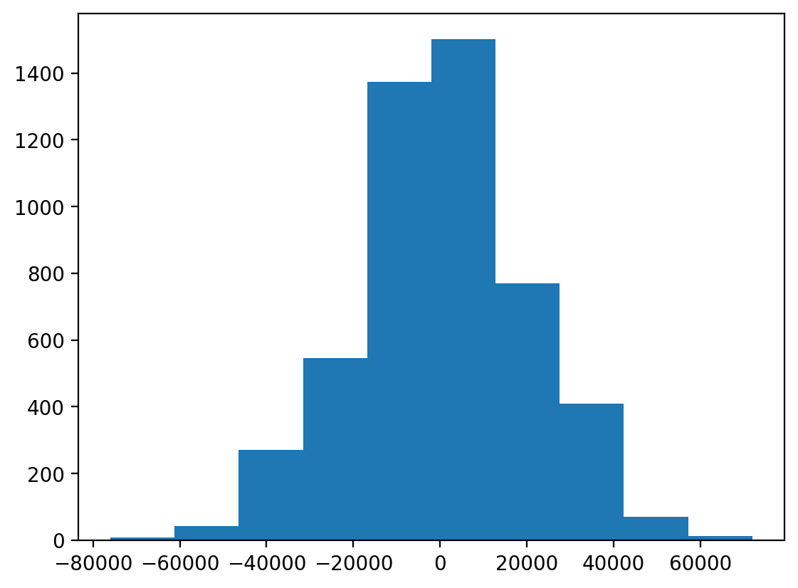
# Plotting cumulative sum of net money won for first 5 players
fig, ax = plt.subplots(figsize=(12, 4))
for i in range(5):
    #win_amount_df.iloc[i].values.cumsum()
    ax.plot(win_amount_df.iloc[i].values.cumsum(), lw=1)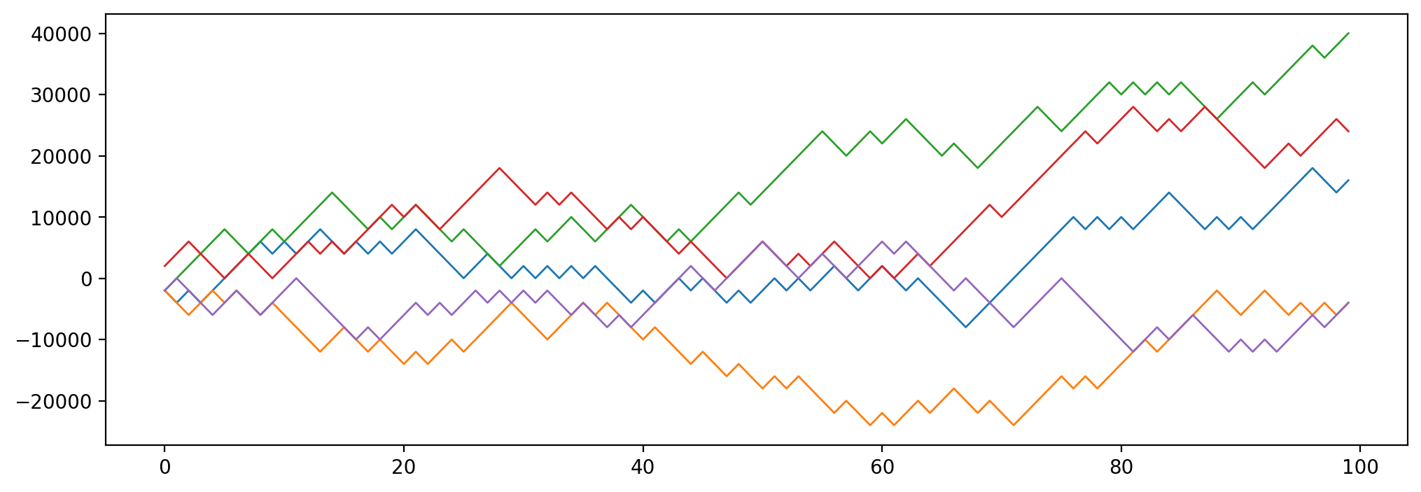
| 0 | 1 | 2 | 3 | 4 | 5 | 6 | 7 | 8 | 9 | ... | 90 | 91 | 92 | 93 | 94 | 95 | 96 | 97 | 98 | 99 | |
|---|---|---|---|---|---|---|---|---|---|---|---|---|---|---|---|---|---|---|---|---|---|
| 0 | -2000.0 | -4000.0 | -2000.0 | -4000.0 | -2000.0 | 0.0 | 2000.0 | 4000.0 | 6000.0 | 4000.0 | ... | 10000.0 | 8000.0 | 10000.0 | 12000.0 | 14000.0 | 16000.0 | 18000.0 | 16000.0 | 14000.0 | 16000.0 |
| 1 | -2000.0 | -4000.0 | -6000.0 | -4000.0 | -2000.0 | -4000.0 | -2000.0 | -4000.0 | -6000.0 | -4000.0 | ... | -6000.0 | -4000.0 | -2000.0 | -4000.0 | -6000.0 | -4000.0 | -6000.0 | -4000.0 | -6000.0 | -4000.0 |
| 2 | -2000.0 | 0.0 | 2000.0 | 4000.0 | 6000.0 | 8000.0 | 6000.0 | 4000.0 | 6000.0 | 8000.0 | ... | 30000.0 | 32000.0 | 30000.0 | 32000.0 | 34000.0 | 36000.0 | 38000.0 | 36000.0 | 38000.0 | 40000.0 |
| 3 | 2000.0 | 4000.0 | 6000.0 | 4000.0 | 2000.0 | 0.0 | 2000.0 | 4000.0 | 2000.0 | 0.0 | ... | 22000.0 | 20000.0 | 18000.0 | 20000.0 | 22000.0 | 20000.0 | 22000.0 | 24000.0 | 26000.0 | 24000.0 |
| 4 | -2000.0 | 0.0 | -2000.0 | -4000.0 | -6000.0 | -4000.0 | -2000.0 | -4000.0 | -6000.0 | -4000.0 | ... | -10000.0 | -12000.0 | -10000.0 | -12000.0 | -10000.0 | -8000.0 | -6000.0 | -8000.0 | -6000.0 | -4000.0 |
5 rows × 100 columns
fig = plt.figure(figsize=(14, 6))
gs = fig.add_gridspec(1, 2, width_ratios=[4, 1])  # 4:1 ratio for main plot and histogram

# Main plot (left plot for cumulative sum)
ax1 = fig.add_subplot(gs[0])
cumsum_df = win_amount_df.cumsum(axis=1)
cumsum_df.T.plot(legend=False, lw=1, alpha=0.1, color='k', ax=ax1)
ax1.set_xlabel("Number of coin flips")
ax1.set_ylabel("Net money won")

# Right plot (histogram)
ax2 = fig.add_subplot(gs[1])
ax2.hist(net_money_won, color='gray', alpha=0.5, orientation='horizontal', bins=30)
ax2.set_xlabel("Frequency")

# Adjust layout
plt.tight_layout()
plt.savefig('coin_flip_game.png', dpi=600)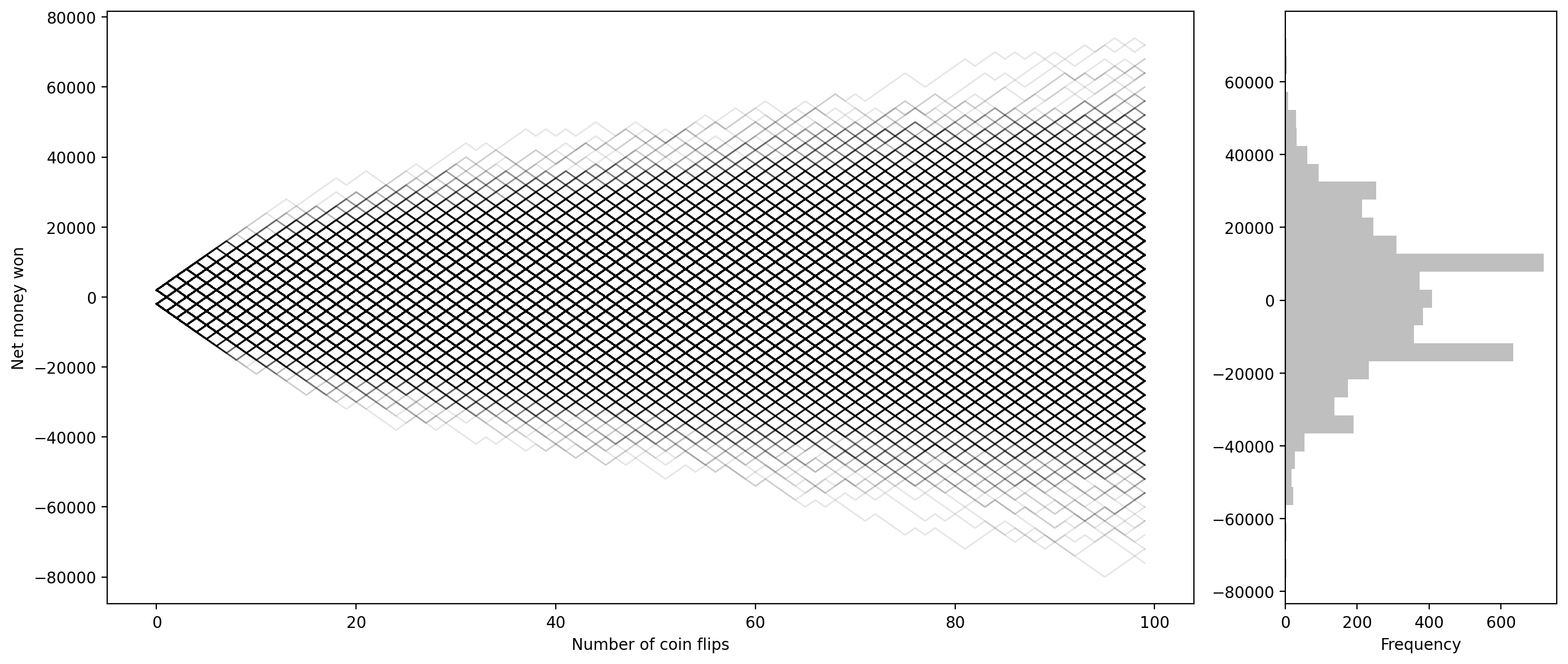

### Finding the mean of Gaussian distrubution

y_lin = torch.linspace(-10, 10, 1000)
sigma = 2.0

out = y_lin*torch.exp(-y_lin**2/(2*sigma**2))
plt.plot(y_lin, out)

# Drawing coordinate axis at x = 0, y = 0
plt.axhline(0, color='black', lw=0.5)
plt.axvline(0, color='black', lw=0.5)

plt.fill_between(y_lin, out, color='gray', alpha=0.5)