Joint Distribution Properties

Exploring properties of joint probability distributions, including independence, covariance, correlation, and bivariate normal distributions with practical examples

Keywords

joint distributions, independence, covariance, correlation, bivariate normal, uniform distribution, PyTorch

import matplotlib.pyplot as plt
import numpy as np
print(np.__version__)
import torch 
import torch.nn as nn

import pandas as pd
# Retina mode
%matplotlib inline
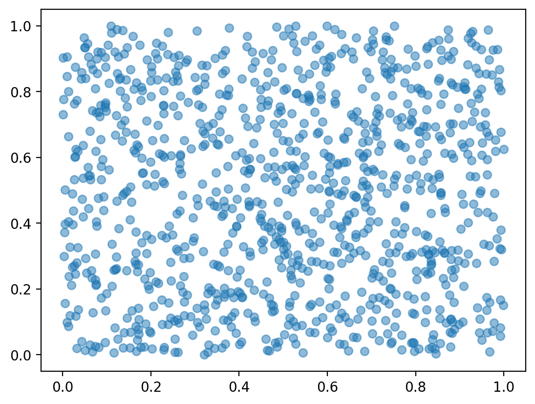
%config InlineBackend.figure_format = 'retina'

1.26.4

X = torch.distributions.Uniform(-1, 1)
Y = torch.distributions.Uniform(-1, 1)

x_samples = X.sample((1000,))
y_samples = Y.sample((1000,))

plt.scatter(x_samples, y_samples)
# aspect ratio
plt.gca().set_aspect('equal')
plt.xlabel('X')
plt.ylabel('Y')

Text(0, 0.5, 'Y')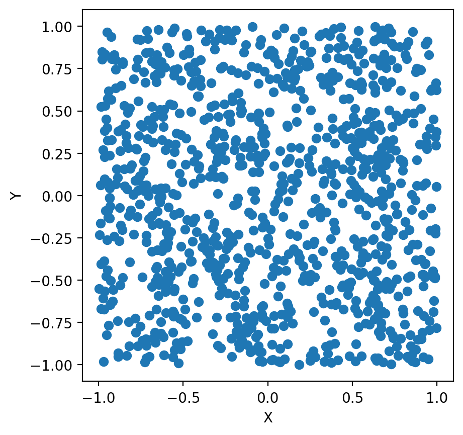

## E[XY] between U(-1, 1) and U(-1, 1)

E_XY = torch.mean(x_samples * y_samples)
print(E_XY)

tensor(-0.0064)

Analytical solution for the expected value of the product of two random variables: \(X\sim U(0,1)\) and \(Y\sim U(0,1)\).

We know that \(f_{X, Y}(x, y) = 1\) for \(0 \leq x \leq 1\) and \(0 \leq y \leq 1\). The expected value of the product of two random variables is given by:

\[\begin{equation} \begin{aligned} E[XY] &= \int_{0}^{1} \int_{0}^{1} xy \, dx \, dy \\ &= \int_{0}^{1} \left[ \frac{1}{2}x^2y \right]_{0}^{1} \, dy \\ &= \int_{0}^{1} \frac{1}{2}y \, dy \\ &= \left[ \frac{1}{4}y^2 \right]_{0}^{1} \\ &= \frac{1}{4} \end{aligned} \end{equation}\]

def E_XY(X, Y, n=1000):
    x_samples = X.sample((n,))
    y_samples = Y.sample((n,))
    return torch.mean(x_samples * y_samples)

X = torch.distributions.Uniform(0, 1)
Y = torch.distributions.Uniform(0, 1)

print(E_XY(X, Y, 1000000))

# This is the same as E[XY] = E[X]E[Y] for independent random variables

tensor(0.2502)

Finding \(\cos(\theta)\) for \(X\sim U(0,1)\) and \(Y\sim U(0,1)\):

\(E[X^2] = \int_{0}^{1} x^2 \, dx = \left[ \frac{1}{3}x^3 \right]_{0}^{1} = \frac{1}{3}\)

\(\cos(\theta) = \frac{E[XY]}{\sqrt{E[X^2]E[Y^2]}} = \frac{\frac{1}{4}}{\sqrt{\frac{1}{3}\frac{1}{3}}} = \frac{3}{4}\)

For any general \(X\sim U(a,b)\) and \(Y\sim U(a,b)\), the expected value of the product of two random variables is given by:

\[\begin{equation} \begin{aligned} E[XY] &= \int_{a}^{b} \int_{a}^{b} xy \, dx \, dy \\ &= \int_{a}^{b} \left[ \frac{1}{2}x^2y \right]_{a}^{b} \, dy \\ &= \int_{a}^{b} \frac{1}{2}(b^2 - a^2)y \, dy \\ &= \frac{1}{2}(b^2 - a^2) \int_{a}^{b} y \, dy \\ &= \frac{1}{2}(b^2 - a^2) \left[ \frac{1}{2}y^2 \right]_{a}^{b} \\ &= \frac{1}{2}(b^2 - a^2) \left( \frac{1}{2}b^2 - \frac{1}{2}a^2 \right) \\ &= \frac{1}{4}(b^2 - a^2)(b^2 - a^2) \\ &= \frac{1}{4}(b - a)^2(b + a)^2 \end{aligned} \end{equation}\]

\(E[X^2] = \int_{a}^{b} x^2 \, dx = \left[ \frac{1}{3}x^3 \right]_{a}^{b} = \frac{1}{3}(b^3 - a^3)\)

\(\sqrt{E[X^2]E[Y^2]} = \sqrt{\frac{1}{3}(b^3 - a^3)\frac{1}{3}(b^3 - a^3)} = \frac{1}{3}(b^3 - a^3)\)

And \(\cos(\theta)\) for \(X\sim U(a,b)\) and \(Y\sim U(a,b)\) is given by:

\[\begin{equation} \begin{aligned} \cos(\theta) &= \frac{E[XY]}{\sqrt{E[X^2]E[Y^2]}} \\ &= \frac{\frac{1}{4}(b - a)^2(b + a)^2}{\frac{1}{3}(b^3 - a^3)} \\ \end{aligned} \end{equation}\]

### cos(theta)

def E_cos_theta(X, Y, n=1000):
    x_samples = X.sample((n,))
    y_samples = Y.sample((n,))
    EXY = torch.mean(x_samples * y_samples)
    EX2 = torch.mean(x_samples ** 2)
    EY2 = torch.mean(y_samples ** 2)
    print(EXY, EX2, EY2)

    return EXY / torch.sqrt(EX2 * EY2)

X = torch.distributions.Uniform(0, 1)
Y = torch.distributions.Uniform(0, 1)

print(E_cos_theta(X, Y, 10000))

tensor(0.2479) tensor(0.3288) tensor(0.3344)
tensor(0.7475)

# Now increasing the range of the random variables
X = torch.distributions.Uniform(10, 11)
Y = torch.distributions.Uniform(10, 11)

print(E_XY(X, Y))

EX2 = torch.mean(x_samples ** 2)
EY2 = torch.mean(y_samples ** 2)

print(EX2, EY2)

tensor(110.4675)
tensor(0.3374) tensor(0.3341)

X = torch.distributions.Uniform(10, 11)
Y = torch.distributions.Uniform(10, 11)

print(E_cos_theta(X, Y, 10000))

tensor(110.3001) tensor(110.3019) tensor(110.4660)
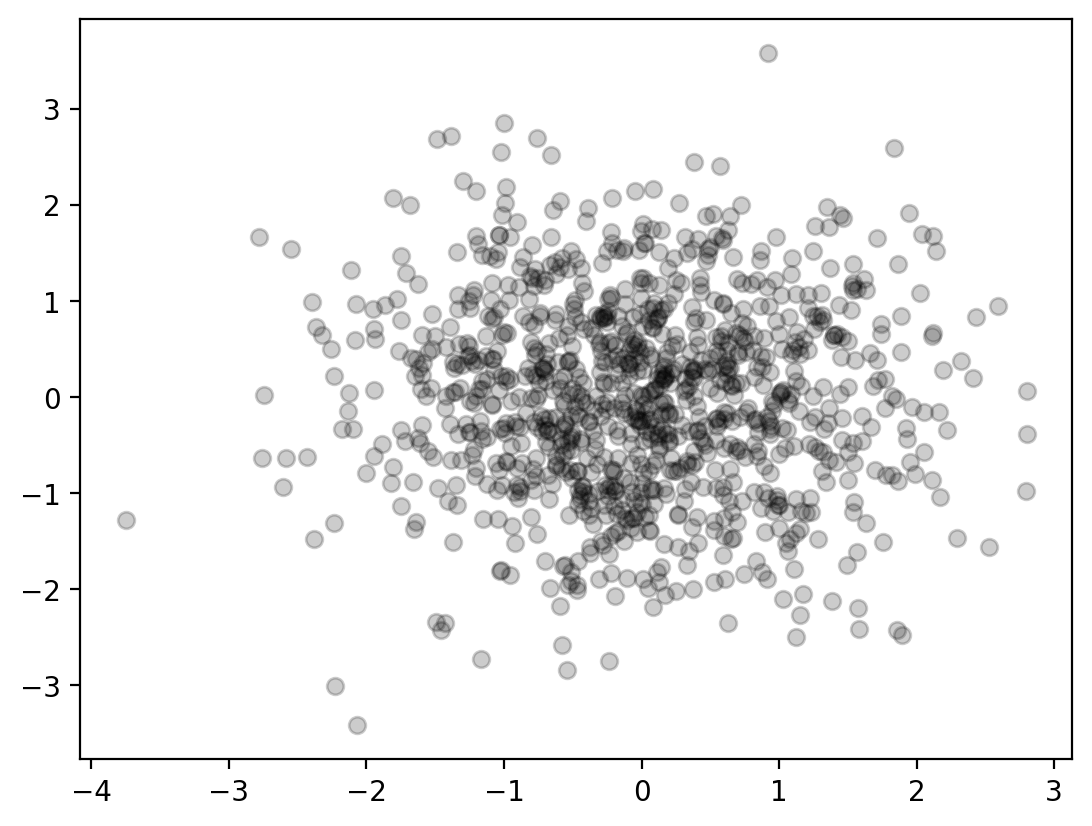
tensor(0.9992)

## E[XY] between N(0, 1) and N(0, 1)

X = torch.distributions.Normal(0, 1)
Y = torch.distributions.Normal(0, 1)

x_samples = X.sample((1000,))
y_samples = Y.sample((1000,))

plt.scatter(x_samples, y_samples)
# aspect ratio
plt.gca().set_aspect('equal')
plt.xlabel('X')
plt.ylabel('Y')

E_XY = torch.mean(x_samples * y_samples)
print(E_XY)

tensor(0.0701)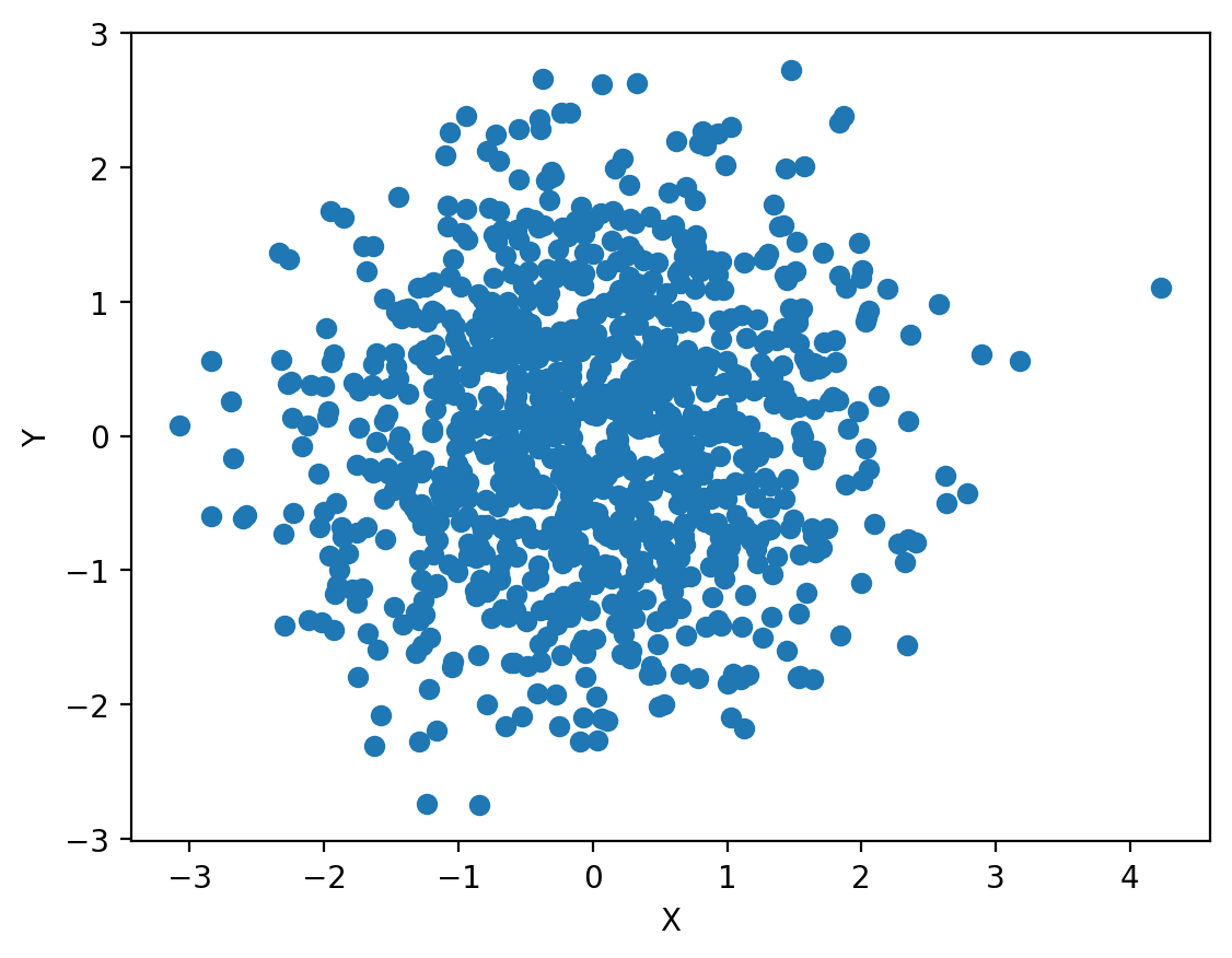

dist = torch.distributions.Normal(0, 1)
x = dist.sample((1000,))
plt.hist(x.numpy(), bins=50, density=True)

x_range = torch.linspace(-3, 3, 1000)
y = dist.log_prob(x_range).exp()
plt.plot(x_range.numpy(), y.numpy())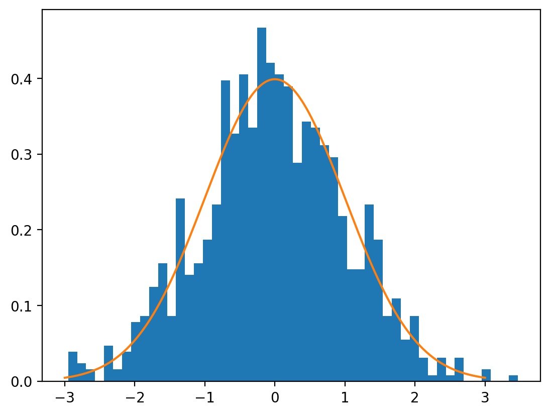

dist.sample([10])

tensor([-1.9083,  0.3758,  0.0051,  0.5140,  0.9852, -0.5989,  0.5222, -0.7744,
         0.9462, -1.7868])

dist_2d_normal = torch.distributions.MultivariateNormal(torch.tensor([0.0, 0.0]), torch.eye(2))
#dist_2d_normal = torch.distributions.MultivariateNormal(torch.tensor([0.0, 0.0]), torch.tensor([[1.0, 0.5], [0.5, 1.0]]))

dist_2d_normal.sample([10])

tensor([[ 0.0438, -0.0310],
        [ 0.0487, -0.3790],
        [-0.7872,  0.9880],
        [ 1.0010, -0.9025],
        [ 0.5449,  0.1047],
        [ 1.6466,  0.0925],
        [ 0.9357,  0.2228],
        [-1.2721,  2.5194],
        [-0.3306, -0.1152],
        [ 1.2249, -1.7330]])

plt.scatter(*dist_2d_normal.sample([1000]).numpy().T, alpha=0.2, color='k')

# Plot 2D normal distribution surface plot of PDF
from mpl_toolkits.mplot3d import Axes3D

x = torch.linspace(-3, 3, 100)
y = torch.linspace(-3, 3, 100)

X, Y = torch.meshgrid(x, y)
xy = torch.stack([X, Y], 2)
z = dist_2d_normal.log_prob(xy).exp()

fig = plt.figure()
ax = fig.add_subplot(111, projection='3d')
ax.plot_surface(X.numpy(), Y.numpy(), z.numpy())

ax.set_xlabel('X')
ax.set_ylabel('Y')
ax.set_zlabel('PDF')

fig.tight_layout()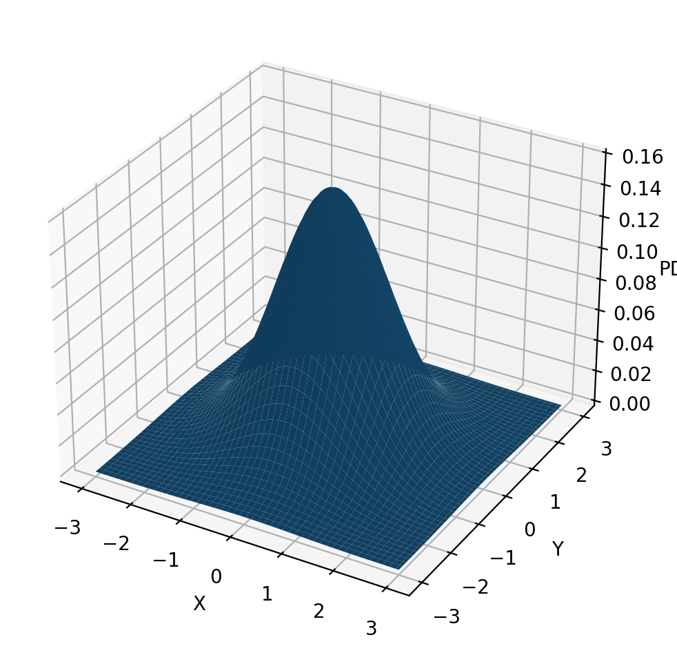

df = pd.read_html("http://socr.ucla.edu/docs/resources/SOCR_Data/SOCR_Data_Dinov_020108_HeightsWeights.html")

store_df = df[0]
store_df.columns = store_df.iloc[0]
store_df = store_df.iloc[1:]
store_df = store_df.astype(float)
store_df = store_df.drop(columns=["Index"])
store_df = store_df.dropna()

store_df.head()

	Height(Inches)	Weight(Pounds)
1	65.78331	112.9925
2	71.51521	136.4873
3	69.39874	153.0269
4	68.21660	142.3354
5	67.78781	144.2971

### Fiting a bi-variate normal distribution to the data
data = torch.tensor(store_df.values)
mean = data.mean(0)
cov = torch.cov(data.T)
dist = torch.distributions.MultivariateNormal(mean, cov)

dist.loc

tensor([ 67.9931, 127.0794], dtype=torch.float64)

dist.covariance_matrix

tensor([[  3.6164,  11.1510],
        [ 11.1510, 135.9765]], dtype=torch.float64)

# Plot the data

plt.scatter(data[:, 0], data[:, 1], alpha=0.1, color='k', facecolors='k')
plt.xlabel("Height")
plt.ylabel("Weight")

Text(0, 0.5, 'Weight')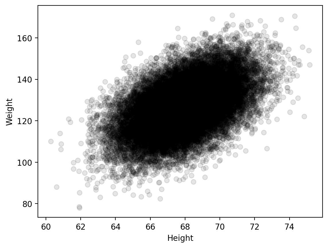

# plot the PDF
x = torch.linspace(50, 80, 100)
y = torch.linspace(80, 280, 100)
X, Y = torch.meshgrid(x, y)
xy = torch.stack([X, Y], 2)
z = dist.log_prob(xy).exp()

import plotly.graph_objects as go

# Create surface plot with custom hover labels
fig = go.Figure(data=[go.Surface(
    x=X, y=Y, z=z, colorscale="viridis",
    hovertemplate="Height: %{x:0.2f}<br>Weight: %{y:0.2f}<br>PDF: %{z:0.5f}<extra></extra>"
)])

# Maximize figure size and reduce whitespace
fig.update_layout(
    autosize=True,
    width=1200,  # Set wider figure
    height=700,  # Set taller figure
    margin=dict(l=0, r=0, t=40, b=0),  # Remove extra whitespace
    title="2D Gaussian PDF",
    scene=dict(
        xaxis_title="Height",
        yaxis_title="Weight",
        zaxis_title="PDF"
    )
)

# Show plot
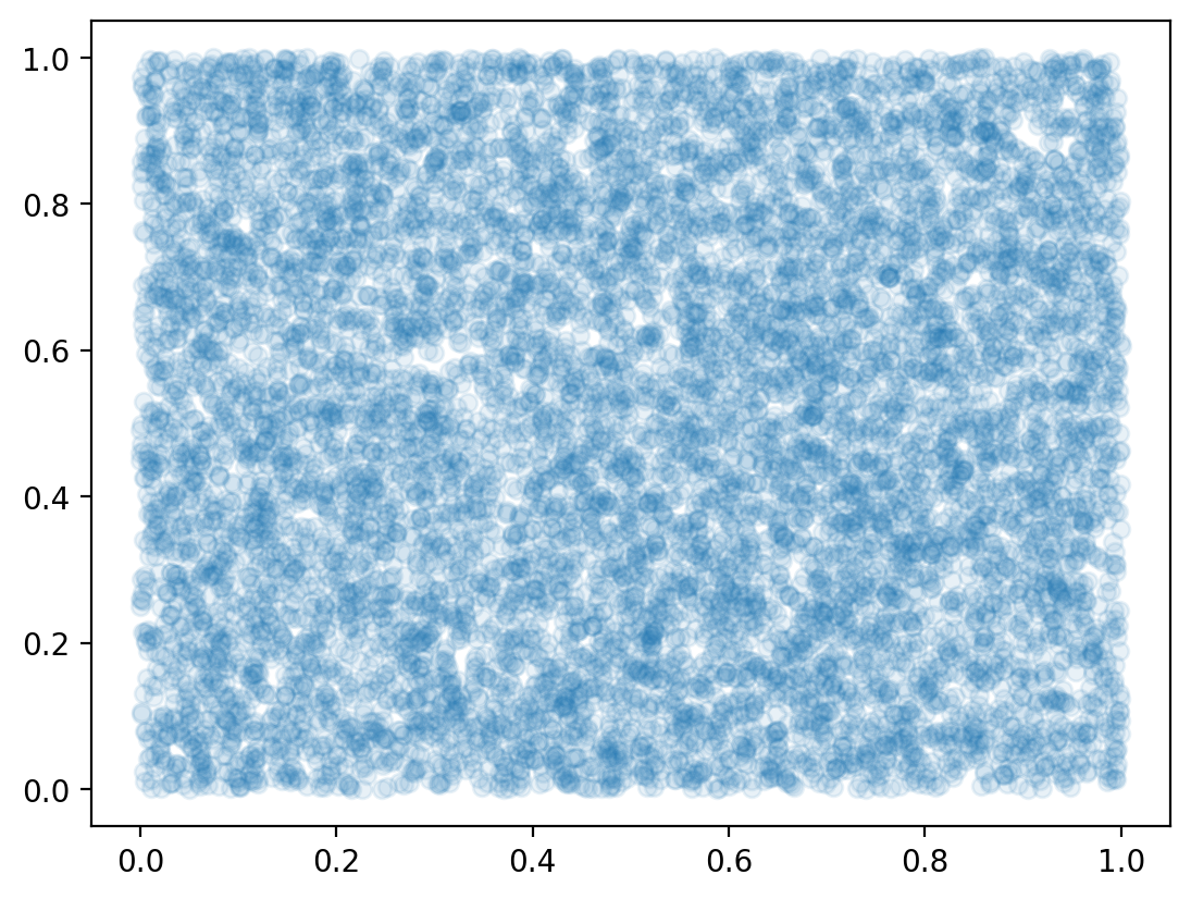
fig.show()

# uniform distribution
dist_uniform = torch.distributions.Uniform(0, 1)
x = dist_uniform.sample((1000,))
plt.hist(x.numpy(), bins=50, density=True)

x_range = torch.linspace(0, 1, 1000)
y = dist_uniform.log_prob(x_range).exp()
plt.plot(x_range.numpy(), y.numpy())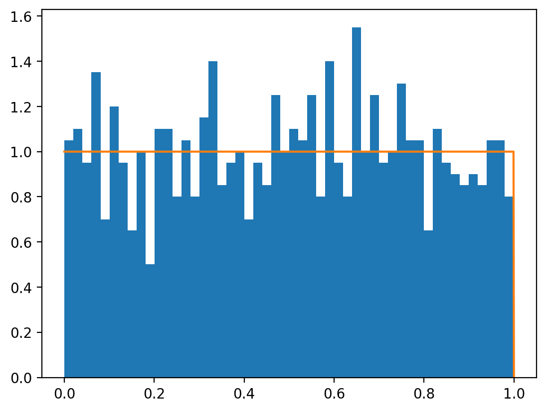

dist_uniform_2d = torch.distributions.Uniform(torch.tensor([0.0, 0.0]), torch.tensor([1.0, 1.0]))
dist_uniform_2d.sample([10])

tensor([[0.5493, 0.3478],
        [0.7661, 0.2568],
        [0.7199, 0.2975],
        [0.9114, 0.2916],
        [0.0045, 0.4948],
        [0.0156, 0.7434],
        [0.6856, 0.1037],
        [0.4446, 0.1913],
        [0.1995, 0.5009],
        [0.0716, 0.6085]])

plt.scatter(*dist_uniform_2d.sample([1000]).numpy().T, alpha=0.5)

plt.scatter(*dist_uniform_2d.sample([10000]).numpy().T, alpha=0.1)

# surface plot of PDF

x = torch.linspace(0.0, 1.0, 100)
y = torch.linspace(0.0, 1.0, 100)

X, Y = torch.meshgrid(x, y)
xy = torch.stack([X, Y], 2)

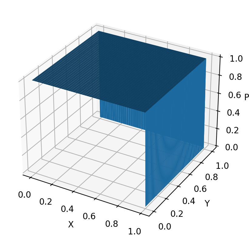
## Important:
## f(x, y) = f(x) * f(y) for independent random variables
## log(f(x, y)) = log(f(x)) + log(f(y))
z1 = dist_uniform_2d.log_prob(xy).sum(-1).exp()
z2 = dist_uniform.log_prob(X).exp() * dist_uniform.log_prob(Y).exp()
assert torch.allclose(z1, z2) 


fig = plt.figure()
ax = fig.add_subplot(111, projection='3d')
ax.plot_surface(X.numpy(), Y.numpy(), z1.numpy())
ax.set_xlabel('X')
ax.set_ylabel('Y')
ax.set_zlabel('PDF')

Text(0.5, 0, 'PDF')