Introduction to Pandas

Author

Nipun Batra, Shreyans Jain, Guntas Singh Saran

Published

January 13, 2025

## 1. Introduction

Pandas is a powerful Python library for data manipulation, offering labeled data structures that make tasks like cleaning, transformation, merging, and analysis more convenient.

import numpy as np
import pandas as pd
import matplotlib.pyplot as plt
import seaborn as sns

print("Using Pandas version:", pd.__version__)
print("Using NumPy version:", np.__version__)
print("Using Seaborn version:", sns.__version__)
%matplotlib inline
%config InlineBackend.figure_format = 'retina'

Using Pandas version: 2.2.3
Using NumPy version: 2.1.2
Using Seaborn version: 0.13.2

2. Numpy vs. Pandas for Student Scores

2.1 Creating and Saving Student Data to Excel/CSV

We’ll first generate some random student data: - Name (string) - Maths (integer) - Science (integer)

Then we’ll save to both .xlsx and .csv for demonstration.

num_students = 20

student_data = {
    "Name": [
        "Aarav", "Vivaan", "Aditya", "Ananya", "Ishita", "Kabir", "Nisha", "Rohan", "Priya", "Sneha",
        "Aryan", "Meera", "Tanya", "Siddharth", "Neha", "Laksh", "Pooja", "Rahul", "Simran", "Kiran"
    ],
    "Maths": np.random.randint(50, 100, size=num_students),
    "Science": np.random.randint(50, 100, size=num_students),
    "Economics": np.random.randint(50, 100, size=num_students),
}

df_students = pd.DataFrame(student_data)

df_students.to_excel("student_scores.xlsx", index=False)
df_students.to_csv("student_scores.csv", index=False)

df_students.head(10)

	Name	Maths	Science	Economics
0	Aarav	53	56	67
1	Vivaan	94	88	85
2	Aditya	84	65	69
3	Ananya	98	90	96
4	Ishita	72	74	78
5	Kabir	79	56	60
6	Nisha	76	52	99
7	Rohan	71	78	50
8	Priya	76	72	68
9	Sneha	64	92	94

2.2 Reading CSV in NumPy & Basic Analysis

NumPy’s loadtxt can be used to read numeric data easily, but handling mixed types (e.g. strings + numbers) can be trickier. We’ll demonstrate a simple approach:

Read the entire CSV (skipping the header) using np.loadtxt.
We’ll parse the Name column as a string and the three score columns as integers.
Compute the mean of Maths and Science.
Find which student got the maximum in Science.
Find which student got the maximum of |Maths - Science|.

!head student_scores.csv

Name,Maths,Science,Economics
Aarav,53,56,67
Vivaan,94,88,85
Aditya,84,65,69
Ananya,98,90,96
Ishita,72,74,78
Kabir,79,56,60
Nisha,76,52,99
Rohan,71,78,50
Priya,76,72,68

data = np.loadtxt("student_scores.csv", delimiter = ",", skiprows = 1, dtype = str)
print(data)

[['Aarav' '53' '56' '67']
 ['Vivaan' '94' '88' '85']
 ['Aditya' '84' '65' '69']
 ['Ananya' '98' '90' '96']
 ['Ishita' '72' '74' '78']
 ['Kabir' '79' '56' '60']
 ['Nisha' '76' '52' '99']
 ['Rohan' '71' '78' '50']
 ['Priya' '76' '72' '68']
 ['Sneha' '64' '92' '94']
 ['Aryan' '60' '92' '97']
 ['Meera' '62' '56' '89']
 ['Tanya' '70' '78' '88']
 ['Siddharth' '73' '72' '83']
 ['Neha' '79' '85' '95']
 ['Laksh' '68' '62' '88']
 ['Pooja' '63' '62' '57']
 ['Rahul' '81' '63' '67']
 ['Simran' '69' '98' '78']
 ['Kiran' '85' '82' '95']]

print(data.dtype)

<U9

names = data[:, 0].tolist()
maths_np = np.array(data[:, 1].astype(int))
science_np = np.array(data[:, 2].astype(int))
eco_np = np.array(data[:, 3].astype(int))

print("Names:", names)
print("Maths scores:", maths_np)
print("Science scores:", science_np)
print("Economics scores:", eco_np)

Names: ['Aarav', 'Vivaan', 'Aditya', 'Ananya', 'Ishita', 'Kabir', 'Nisha', 'Rohan', 'Priya', 'Sneha', 'Aryan', 'Meera', 'Tanya', 'Siddharth', 'Neha', 'Laksh', 'Pooja', 'Rahul', 'Simran', 'Kiran']
Maths scores: [53 94 84 98 72 79 76 71 76 64 60 62 70 73 79 68 63 81 69 85]
Science scores: [56 88 65 90 74 56 52 78 72 92 92 56 78 72 85 62 62 63 98 82]
Economics scores: [67 85 69 96 78 60 99 50 68 94 97 89 88 83 95 88 57 67 78 95]

print(type(maths_np))
print(maths_np.dtype)

<class 'numpy.ndarray'>
int64

mean_maths = np.mean(maths_np)
mean_science = np.mean(science_np)
mean_eco = np.mean(eco_np)

print(f"\nMean Maths score: {mean_maths:.3f}")
print(f"Mean Science score: {mean_science:.3f}")
print(f"Mean Economics score: {mean_eco:.3f}")

print(f"\nMean Maths score (integer): {mean_maths:.2f}")


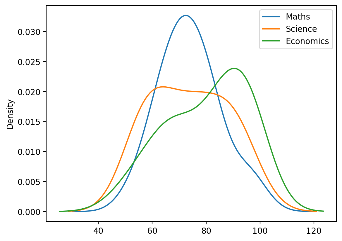
Mean Maths score: 73.850
Mean Science score: 73.650
Mean Economics score: 80.150

Mean Maths score (integer): 73.85

# Finding student with maximum science
max_sci_idx = np.argmax(science_np)
print(max_sci_idx)

# since we need the name of the student, we use the index (from argmax) to find the name
max_sci_student = names[max_sci_idx]
max_sci_val = science_np[max_sci_idx]
print(f"\nStudent with maximum science score: {max_sci_student} ({max_sci_val})")


Student with maximum science score: Simran (98)

# Likewise for finding student with maximum |Maths - Science| score
diff = np.abs(maths_np - science_np)
max_diff_idx = np.argmax(diff)
max_diff_student = names[max_diff_idx]
print(f"\nStudent with max |Maths - Science|: {max_diff_student} (|{maths_np[max_diff_idx]} - {science_np[max_diff_idx]}| = {diff[max_diff_idx]})")


Student with max |Maths - Science|: Aryan (|60 - 92| = 32)

2.3 Plotting Student Scores with NumPy/Seaborn

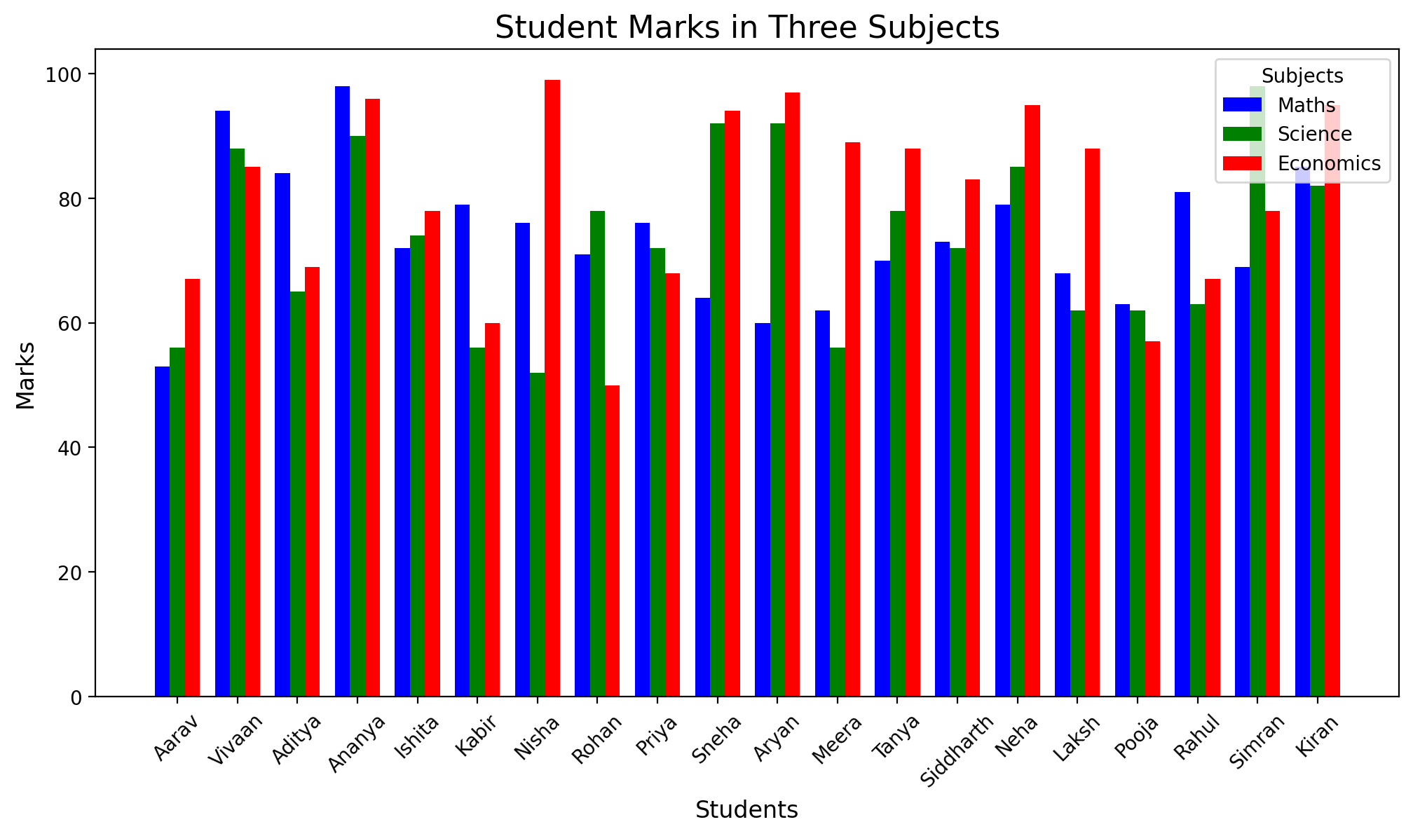
# Define bar width and positions
bar_width = 0.25
x = np.arange(len(names))

# Create the figure and axis
fig, ax = plt.subplots(figsize=(12, 6))

# Plot the bars
ax.bar(x - bar_width, maths_np, width=bar_width, label="Maths", color='blue')
ax.bar(x, science_np, width=bar_width, label="Science", color='green')
ax.bar(x + bar_width, eco_np, width=bar_width, label="Economics", color='red')

# Customize the plot
ax.set_title("Student Marks in Three Subjects", fontsize=16)
ax.set_xlabel("Students", fontsize=12)
ax.set_ylabel("Marks", fontsize=12)
ax.set_xticks(x)
ax.set_xticklabels(names, rotation=45)
ax.legend(title="Subjects")

### 2.4 Reading CSV in Pandas & Repeating Analysis With Pandas, we can directly do:

df = pd.read_csv("student_scores.csv")

and the DataFrame will automatically separate columns into name, maths, and science. Then we can easily compute means, maxima, etc.

df_students_pandas = pd.read_csv("student_scores.csv")
df_students_pandas

	Name	Maths	Science	Economics
0	Aarav	53	56	67
1	Vivaan	94	88	85
2	Aditya	84	65	69
3	Ananya	98	90	96
4	Ishita	72	74	78
5	Kabir	79	56	60
6	Nisha	76	52	99
7	Rohan	71	78	50
8	Priya	76	72	68
9	Sneha	64	92	94
10	Aryan	60	92	97
11	Meera	62	56	89
12	Tanya	70	78	88
13	Siddharth	73	72	83
14	Neha	79	85	95
15	Laksh	68	62	88
16	Pooja	63	62	57
17	Rahul	81	63	67
18	Simran	69	98	78
19	Kiran	85	82	95

df_students_pandas.describe()

	Maths	Science	Economics
count	20.000000	20.000000	20.000000
mean	73.850000	73.650000	80.150000
std	11.230949	14.224793	14.928866
min	53.000000	52.000000	50.000000
25%	67.000000	62.000000	67.750000
50%	72.500000	73.000000	84.000000
75%	79.500000	85.750000	94.250000
max	98.000000	98.000000	99.000000

!head student_scores.csv

Name,Maths,Science,Economics
Aarav,53,56,67
Vivaan,94,88,85
Aditya,84,65,69
Ananya,98,90,96
Ishita,72,74,78
Kabir,79,56,60
Nisha,76,52,99
Rohan,71,78,50
Priya,76,72,68

df_students_pandas.head?

Signature: df_students_pandas.head(n: 'int' = 5) -> 'Self'
Docstring:
Return the first `n` rows.
This function returns the first `n` rows for the object based
on position. It is useful for quickly testing if your object
has the right type of data in it.
For negative values of `n`, this function returns all rows except
the last `|n|` rows, equivalent to ``df[:n]``.
If n is larger than the number of rows, this function returns all rows.
Parameters
----------
n : int, default 5
    Number of rows to select.
Returns
-------
same type as caller
    The first `n` rows of the caller object.
See Also
--------
DataFrame.tail: Returns the last `n` rows.
Examples
--------
>>> df = pd.DataFrame({'animal': ['alligator', 'bee', 'falcon', 'lion',
...                    'monkey', 'parrot', 'shark', 'whale', 'zebra']})
>>> df
      animal
0  alligator
1        bee
2     falcon
3       lion
4     monkey
5     parrot
6      shark
7      whale
8      zebra
Viewing the first 5 lines
>>> df.head()
      animal
0  alligator
1        bee
2     falcon
3       lion
4     monkey
Viewing the first `n` lines (three in this case)
>>> df.head(3)
      animal
0  alligator
1        bee
2     falcon
For negative values of `n`
>>> df.head(-3)
      animal
0  alligator
1        bee
2     falcon
3       lion
4     monkey
5     parrot
File:      ~/mambaforge/lib/python3.12/site-packages/pandas/core/generic.py
Type:      method

df_students_pandas.head(n=10)

	Name	Maths	Science	Economics
0	Aarav	53	56	67
1	Vivaan	94	88	85
2	Aditya	84	65	69
3	Ananya	98	90	96
4	Ishita	72	74	78
5	Kabir	79	56	60
6	Nisha	76	52	99
7	Rohan	71	78	50
8	Priya	76	72	68
9	Sneha	64	92	94

df_students_pandas.tail()

	Name	Maths	Science	Economics
15	Laksh	68	62	88
16	Pooja	63	62	57
17	Rahul	81	63	67
18	Simran	69	98	78
19	Kiran	85	82	95

# Displaying the indices and columns
print(f"Indices: {df_students_pandas.index}")
print(f"Columns: {df_students_pandas.columns}")

Indices: RangeIndex(start=0, stop=20, step=1)
Columns: Index(['Name', 'Maths', 'Science', 'Economics'], dtype='object')

# Displaying the data types of each column
print("\nData Info:")
df_students_pandas.info()


Data Info:
<class 'pandas.core.frame.DataFrame'>
RangeIndex: 20 entries, 0 to 19
Data columns (total 4 columns):
 #   Column     Non-Null Count  Dtype 
---  ------     --------------  ----- 
 0   Name       20 non-null     object
 1   Maths      20 non-null     int64 
 2   Science    20 non-null     int64 
 3   Economics  20 non-null     int64 
dtypes: int64(3), object(1)
memory usage: 772.0+ bytes

# Mean
print("\nMean Maths:", df_students_pandas['Maths'].mean())
print("Mean Science:", df_students_pandas['Science'].mean())


Mean Maths: 73.85
Mean Science: 73.65

# Student with maximum science using different indexing methods
df_students_pandas.loc[df_students_pandas['Science'].idxmax()]

Name         Simran
Maths            69
Science          98
Economics        78
Name: 18, dtype: object

# Student with maximum |Maths - Science|
diff_pd = (df_students_pandas['Maths'] - df_students_pandas['Science']).abs()
max_diff_idx_pd = diff_pd.idxmax()
print("\nStudent with max |Maths - Science|:", df_students_pandas.loc[max_diff_idx_pd, 'Name'], diff_pd[max_diff_idx_pd])


Student with max |Maths - Science|: Aryan 32

Histogram of Student Scores using df.plot()

df_students_pandas.plot.hist(subplots=True, layout=(1, 3), figsize=(18, 6), bins=10, alpha=0.6)

array([[<Axes: ylabel='Frequency'>, <Axes: ylabel='Frequency'>,
        <Axes: ylabel='Frequency'>]], dtype=object)

df_students_pandas.plot.hist(subplots=True, layout=(3, 1), figsize=(6, 9), bins=10, alpha=0.6)

array([[<Axes: ylabel='Frequency'>],
       [<Axes: ylabel='Frequency'>],
       [<Axes: ylabel='Frequency'>]], dtype=object)

df_students_pandas.plot.hist(subplots=False, alpha=0.6)

df_students_pandas.plot.density()

Some more plotting examples with Pandas `df.plot()`

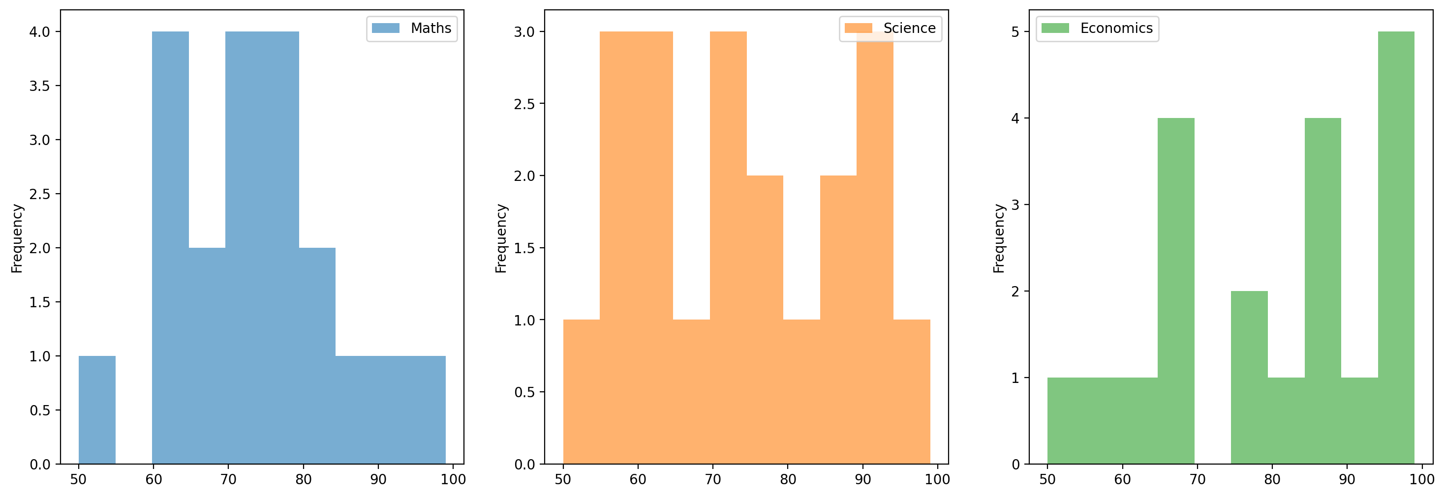
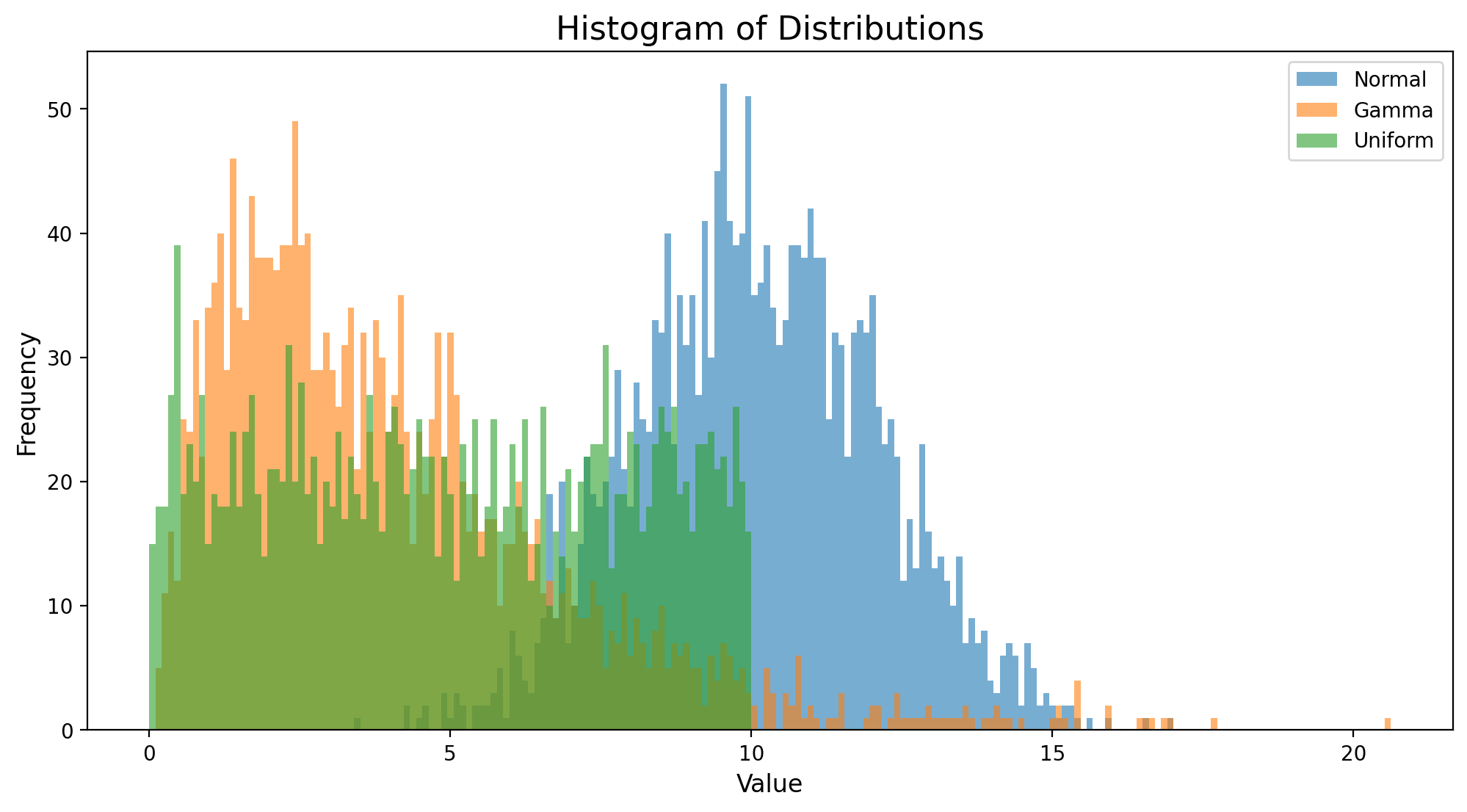
normal = pd.Series(np.random.normal(loc = 10, scale = 2, size = 2000)) # loc is mean, scale is standard deviation
gamma = pd.Series(np.random.gamma(shape = 2, scale = 2, size = 2000)) # shape is k, scale is theta
uniform = pd.Series(np.random.uniform(low = 0, high = 10, size = 2000)) # low is a, high is b

df = pd.DataFrame({'Normal': normal, 'Gamma': gamma, 'Uniform': uniform})
df.head()

	Normal	Gamma	Uniform
0	8.566490	4.439362	2.169578
1	10.946834	5.073406	0.512258
2	7.099340	1.638423	2.346859
3	11.799476	0.733187	2.480262
4	9.174528	4.601980	5.228461

df.plot(kind='hist', bins=200, alpha=0.6, figsize=(12, 6))
plt.title("Histogram of Distributions", fontsize=16)
plt.xlabel("Value", fontsize=12)
plt.ylabel("Frequency", fontsize=12)
plt.show()

Seeing them separately

fig, axes = plt.subplots(1, 3, figsize=(18, 6), sharey=True)
sns.histplot(df['Normal'], bins=100, kde=True, color="skyblue", ax=axes[0])
axes[0].set_title("Normal Distribution", fontsize=14)
sns.histplot(df['Gamma'], bins=100, kde=True, color="salmon", ax=axes[1])
axes[1].set_title("Gamma Distribution", fontsize=14)
sns.histplot(df['Uniform'], bins=100, kde=True, color="limegreen", ax=axes[2])
axes[2].set_title("Uniform Distribution", fontsize=14)

for ax in axes:
    ax.set_xlabel("Value", fontsize=12)
    ax.set_ylabel("Frequency", fontsize=12)

plt.tight_layout()
plt.show()

3. Core Pandas Data Structures

Series

A Series is a one-dimensional labeled array. It can be created from a Python list or NumPy array, optionally providing a custom index. The index labels let you reference elements by name instead of by integer position.

# Creating a Pandas Series
labels = ['a','b','c','d']
data = [10, 0, 50, 40]
ser = pd.Series(data, index=labels, dtype=np.float64)
ser

a    10.0
b     0.0
c    50.0
d    40.0
dtype: float64

# Other methods to create a Pandas Series
d = {'a': 10, 'b': 0, 'c': 50, 'd': 40}
ser = pd.Series(d)
ser

a    10
b     0
c    50
d    40
dtype: int64

# Accessing by label - like a python dictionary
print("\nValue at index 'c':", ser['c'])
print(d['c'])


Value at index 'c': 50
50

# Vectorized ops
print("\nMultiply entire Series by 2:")
ser*2


Multiply entire Series by 2:

a     20
b      0
c    100
d     80
dtype: int64

ser.sort_values()

b     0
a    10
d    40
c    50
dtype: int64

ser

a    10
b     0
c    50
d    40
dtype: int64

ser.sort_values(inplace=True)
ser

b     0
a    10
d    40
c    50
dtype: int64

ser.plot()

ser.sort_index(inplace=True)
ser

a    10
b     0
c    50
d    40
dtype: int64

ser.plot.bar()

ser.plot(kind='bar', rot=0)

ser.plot(kind='barh')

# Accessing by position - like a numpy array
print("\nValue at position 2:", ser.iloc[2])


Value at position 2: 50

ser

a    10
b     0
c    50
d    40
dtype: int64

# Access by key - like a python dictionary
print("\nValue at index 'c':", ser.loc['c'])
print("\nValue at index 'c':", ser['c'])


Value at index 'c': 50

Value at index 'c': 50

ser['c'], ser.loc['c']

(np.int64(50), np.int64(50))

# Access range
print("\nValues in range 1 to 3:")
ser.iloc[1:3]


Values in range 1 to 3:

b     0
c    50
dtype: int64

# access range by label
print("\nValues in range 'b' to 'd':")
ser.loc['b':'d']


Values in range 'b' to 'd':

b     0
c    50
d    40
dtype: int64

# Other methods
ser.describe()

count     4.000000
mean     25.000000
std      23.804761
min       0.000000
25%       7.500000
50%      25.000000
75%      42.500000
max      50.000000
dtype: float64

print(ser.mean(), type(ser.mean()), ser.mean().item(), type(ser.mean().item()))

25.0 <class 'numpy.float64'> 25.0 <class 'float'>

ser

a    10
b     0
c    50
d    40
dtype: int64

ser.rank()

a    2.0
b    1.0
c    4.0
d    3.0
dtype: float64

# Access numpy array from Pandas Series
arr = ser.values
print("\nNumpy array:", arr)
print("Type of array:", type(arr))


Numpy array: [10  0 50 40]
Type of array: <class 'numpy.ndarray'>

ser

a    10
b     0
c    50
d    40
dtype: int64

# Print series where elements are greater than 20
mask = ser > 20
print(mask)

a    False
b    False
c     True
d     True
dtype: bool

ser[mask]

c    50
d    40
dtype: int64

DataFrame

A DataFrame is a 2D tabular data structure with labeled rows (index) and columns. Each column is essentially a Pandas Series.

We can build one from a dictionary of lists, or by reading data from external sources (CSV, SQL, Excel, etc.).

# Creating a DataFrame from a dictionary
data_dict = {
    'Name': ['Alice', 'Bob', 'Charlie'],
    'Age': [24, 42, 18],
    'Score': [88.5, 93.0, 78.0]
}
df = pd.DataFrame(data_dict)
df.index = df['Name']
df = df.drop(['Name'], axis=1)
df

	Age	Score
Name
Alice	24	88.5
Bob	42	93.0
Charlie	18	78.0

df.plot(kind='bar')

data_dict = {
    'Name': ['Alice', 'Bob', 'Charlie'],
    'Age': [24, 42, 18],
    'Score': [88.5, 93.0, 78.0]
}
df = pd.DataFrame(data_dict)
df

	Name	Age	Score
0	Alice	24	88.5
1	Bob	42	93.0
2	Charlie	18	78.0

4. Indexing & Selection

DataFrame selection can occur by column name, row label/index name (.loc), or row position/numpy-array like indexing (.iloc). Boolean masks also apply.

df[col] => a Series of that column.
df.loc[row_label] => row by label.
df.iloc[row_position] => row by integer position.
Boolean indexing => df[df['Age'] > 20].
Slicing => df.loc['a':'b'], df.iloc[0:2].

df2 = pd.DataFrame({
    'X': np.random.rand(5),
    'Y': np.random.rand(5),
    'Z': np.random.randint(1,10,size=5)
}, index=['a','b','c','d','e'])

df2

	X	Y	Z
a	0.996172	0.280775	7
b	0.578735	0.931498	4
c	0.654491	0.699822	4
d	0.172585	0.014937	9
e	0.858278	0.753386	8

df2

	X	Y	Z
a	0.967366	0.753478	2
b	0.401003	0.238826	6
c	0.157301	0.384844	8
d	0.016926	0.387394	7
e	0.659675	0.817511	4

print("\nSelect column 'Y':")
print(df2['Y'])


Select column 'Y':
a    0.280775
b    0.931498
c    0.699822
d    0.014937
e    0.753386
Name: Y, dtype: float64

type(df2['Y'])

pandas.core.series.Series

print("\nSelect row 'c' using loc:")
display(df2.loc['c'])


Select row 'c' using loc:

X    0.654491
Y    0.699822
Z    4.000000
Name: c, dtype: float64

print("\nSelect row at position 2 using iloc:")
display(df2.iloc[2])


Select row at position 2 using iloc:

X    0.654491
Y    0.699822
Z    4.000000
Name: c, dtype: float64

print("\nBoolean mask: rows where Z > 5")
mask = df2['Z'] > 5
display(df2[mask])


Boolean mask: rows where Z > 5

	X	Y	Z
a	0.996172	0.280775	7
d	0.172585	0.014937	9
e	0.858278	0.753386	8

# loc to address by row, col "names" AND iloc to address by row, col "indices"
print(df2.loc['c', 'Y'], df2.iloc[2, 1])

0.6998221861720456 0.6998221861720456

# Select multiple rows
print("\nSelect rows 'a' and 'c':")
display(df2.loc[['a', 'c']])


Select rows 'a' and 'c':

	X	Y	Z
a	0.996172	0.280775	7
c	0.654491	0.699822	4

# Select multiple columns
print("\nSelect columns 'X' and 'Z':")
display(df2[['X', 'Z']])


Select columns 'X' and 'Z':

	X	Z
a	0.610954	6
b	0.059152	3
c	0.483286	9
d	0.325020	8
e	0.059134	3

# Use loc notation to select multiple column
print("\nSelect columns 'X' and 'Z' using loc:")
#display(df2.loc[:, ['X', 'Z']])


# Select rows 'b' and 'd' and columns 'X' and 'Z'
rows_to_select = ['b', 'd']
cols_to_select = ['X', 'Z']
df2.loc[rows_to_select, cols_to_select]


df2.loc['b':'d', 'Y':'Z']


Select columns 'X' and 'Z' using loc:

	Y	Z
b	0.931498	4
c	0.699822	4
d	0.014937	9

# Select rows and columns
print("\nSelect rows 'b' and 'd', columns 'Y' and 'Z':")
display(df2.loc[['b', 'd'], ['Y', 'Z']])


Select rows 'b' and 'd', columns 'Y' and 'Z':

	Y	Z
b	0.895559	3
d	0.573120	8

5. Merging & Joining Data

Pandas provides efficient ways to combine datasets:

pd.concat([df1, df2]): Stack DataFrames (row or column-wise). Preferred for simple stacking horizontally or vertically.
df1.append(df2): Similar to concat row-wise but less efficient since it involves creation of a new index.
pd.merge(df1, df2, on='key'): Database-style merges. Also left_on, right_on, left_index, right_index.

We can specify how to merge: ‘inner’, ‘outer’, ‘left’, ‘right’.

Concatenation of two dataframes with same columns - just stacks them vertically along with their indices

x = pd.DataFrame({'A': ['A0', 'A1'], 'B': ['B0', 'B1']}, index=[0, 1])
y = pd.DataFrame({'A': ['A2', 'A3'], 'B': ['B2', 'B3']}, index=[0, 1])
df_concat = pd.concat([x, y])
display("x:")
display(x)
display("y:")
display(y)
display("pd.concat([x, y]):")
display(df_concat)

'x:'

	A	B
0	A0	B0
1	A1	B1

'y:'

	A	B
0	A2	B2
1	A3	B3

'pd.concat([x, y]):'

	A	B
0	A0	B0
1	A1	B1
0	A2	B2
1	A3	B3

Having similar indices will result in ambuiguity in addressing the rows, so we need to reset the index or use `ignore_index=True`

df_concat.loc[0]

	A	B
0	A0	B0
0	A2	B2

df = pd.concat([x, y], ignore_index=True)
df

	A	B
0	A0	B0
1	A1	B1
2	A2	B2
3	A3	B3

Example specifying the axis of concatenation - row-wise or column-wise.

z = pd.DataFrame({'C': ['C0', 'C1'], 'D': ['D0', 'D1']}, index=[0, 1])
df_col_combine = pd.concat([x, z], axis='columns')

display("x:")
display(x)
display("z:")
display(z)
display("pd.concat([x, z], axis='columns'):")
display(df_col_combine)

'x:'

	A	B
0	A0	B0
1	A1	B1

'z:'

	C	D
0	C0	D0
1	C1	D1

"pd.concat([x, z], axis='columns'):"

	A	B	C	D
0	A0	B0	C0	D0
1	A1	B1	C1	D1

Let’s use seaborn’s ‘tips’ dataset to demonstrate merges.

tips = sns.load_dataset('tips')  # Load the 'tips' dataset from seaborn
print("'tips' dataset shape:", tips.shape)  # Print the shape (rows, columns) of the dataset
display(tips.head())  # Show the first 5 rows of the dataset

'tips' dataset shape: (244, 7)

	total_bill	tip	sex	smoker	day	time	size
0	16.99	1.01	Female	No	Sun	Dinner	2
1	10.34	1.66	Male	No	Sun	Dinner	3
2	21.01	3.50	Male	No	Sun	Dinner	3
3	23.68	3.31	Male	No	Sun	Dinner	2
4	24.59	3.61	Female	No	Sun	Dinner	4

is_vip = np.random.choice([True, False], size=len(tips))  # Randomly assign VIP status (True/False) to each row

customer_ids = np.arange(1, len(tips) + 1)  # Create unique customer IDs starting from 1
np.random.shuffle(customer_ids)  # Shuffle the customer IDs randomly

vip_info = pd.DataFrame({
    'customer_id': customer_ids,  # Assign customer IDs
    'vip': is_vip  # Assign the corresponding VIP status
})

print("VIP info:")
display(vip_info)  # Display the VIP information table

VIP info:

	customer_id	vip
0	119	True
1	148	True
2	2	True
3	84	True
4	76	False
...	...	...
239	218	True
240	146	True
241	176	True
242	164	False
243	19	True

244 rows × 2 columns

tips_ext = tips.copy()  # Create a copy of the original 'tips' dataset
new_customer_ids = np.arange(1, len(tips) + 1)  # Generate new unique customer IDs
np.random.shuffle(new_customer_ids)  # Shuffle the customer IDs randomly

tips_ext['customer_id'] = new_customer_ids  # Add the shuffled customer IDs as a new column
print("Extended tips:")
display(tips_ext)  # Show the extended dataset

Extended tips:

	total_bill	tip	sex	smoker	day	time	size	customer_id
0	16.99	1.01	Female	No	Sun	Dinner	2	32
1	10.34	1.66	Male	No	Sun	Dinner	3	22
2	21.01	3.50	Male	No	Sun	Dinner	3	136
3	23.68	3.31	Male	No	Sun	Dinner	2	137
4	24.59	3.61	Female	No	Sun	Dinner	4	156
...	...	...	...	...	...	...	...	...
239	29.03	5.92	Male	No	Sat	Dinner	3	228
240	27.18	2.00	Female	Yes	Sat	Dinner	2	84
241	22.67	2.00	Male	Yes	Sat	Dinner	2	219
242	17.82	1.75	Male	No	Sat	Dinner	2	241
243	18.78	3.00	Female	No	Thur	Dinner	2	209

244 rows × 8 columns

merged = pd.merge(tips_ext, vip_info, on='customer_id', how='left')  # Merge the datasets using 'customer_id'
print("Merged Data:")
display(merged)  # Display the merged dataset

Merged Data:

	total_bill	tip	sex	smoker	day	time	size	customer_id	vip
0	16.99	1.01	Female	No	Sun	Dinner	2	32	True
1	10.34	1.66	Male	No	Sun	Dinner	3	22	False
2	21.01	3.50	Male	No	Sun	Dinner	3	136	True
3	23.68	3.31	Male	No	Sun	Dinner	2	137	True
4	24.59	3.61	Female	No	Sun	Dinner	4	156	False
...	...	...	...	...	...	...	...	...	...
239	29.03	5.92	Male	No	Sat	Dinner	3	228	False
240	27.18	2.00	Female	Yes	Sat	Dinner	2	84	True
241	22.67	2.00	Male	Yes	Sat	Dinner	2	219	False
242	17.82	1.75	Male	No	Sat	Dinner	2	241	True
243	18.78	3.00	Female	No	Thur	Dinner	2	209	True

244 rows × 9 columns

6. GroupBy & Aggregation

The GroupBy abstraction splits data into groups, applies operations, then combines results. Common for summarizing numeric columns by categories.

Example with tips data

We’ll group by day of the week and compute average tip, total tip, etc.

tips.loc[:, 'day']

0       Sun
1       Sun
2       Sun
3       Sun
4       Sun
       ... 
239     Sat
240     Sat
241     Sat
242     Sat
243    Thur
Name: day, Length: 244, dtype: category
Categories (4, object): ['Thur', 'Fri', 'Sat', 'Sun']

tips['day'].value_counts()

day
Sat     87
Sun     76
Thur    62
Fri     19
Name: count, dtype: int64

# Unique values in the 'day' column
unique_days = tips['day'].unique()
print("Unique days:", unique_days)

Unique days: ['Sun', 'Sat', 'Thur', 'Fri']
Categories (4, object): ['Thur', 'Fri', 'Sat', 'Sun']

mask = tips['day'] == 'Sun'
mask

0       True
1       True
2       True
3       True
4       True
       ...  
239    False
240    False
241    False
242    False
243    False
Name: day, Length: 244, dtype: bool

tips[mask]['tip'].mean().item()

3.2551315789473687

out = {}
for day in unique_days:
    mask = tips['day'] == day
    out[day] = tips[mask]['tip'].mean().item()

out

{'Sun': 3.2551315789473687,
 'Sat': 2.993103448275862,
 'Thur': 2.771451612903225,
 'Fri': 2.7347368421052627}

ser = pd.Series(out)
ser.plot(kind='bar')

grpby = tips.groupby('day', observed=True)['tip']
grpby.mean()

day
Thur    2.771452
Fri     2.734737
Sat     2.993103
Sun     3.255132
Name: tip, dtype: float64

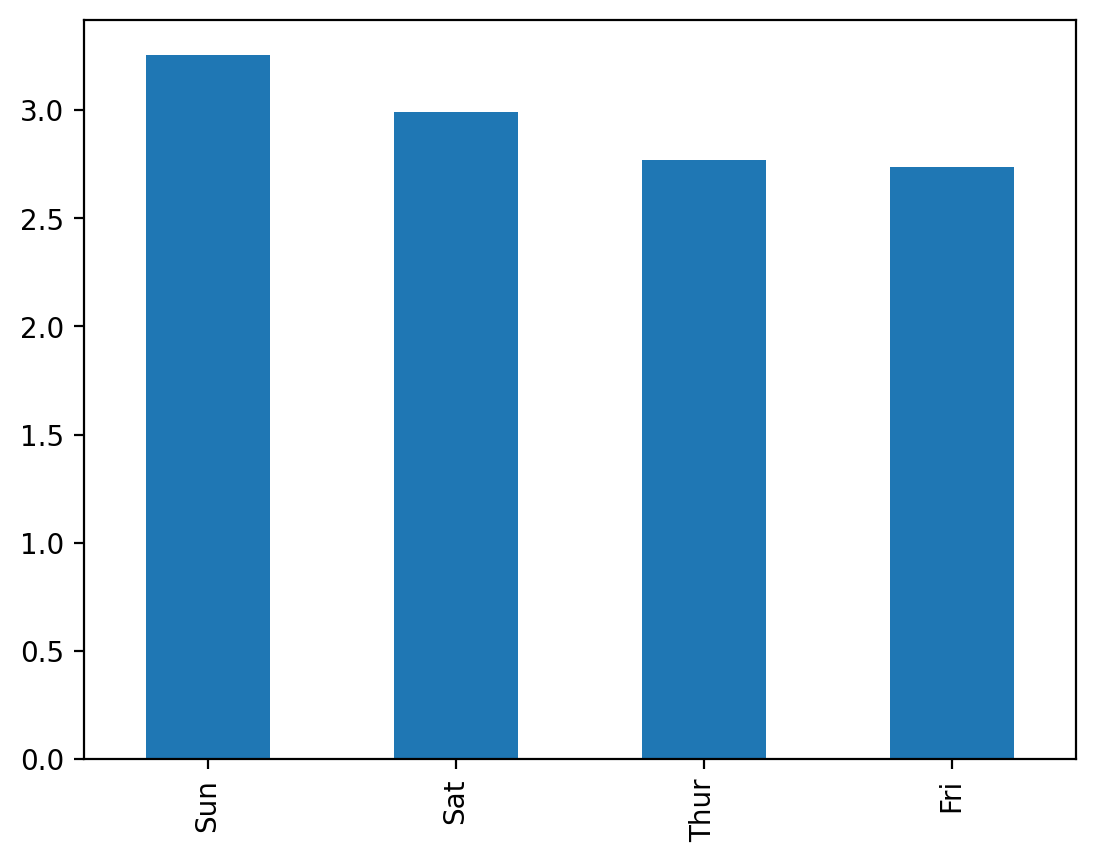
# Group tips by 'day' column, aggregate 'tip' in different ways
grouped = tips.groupby('day', observed=True)['tip']
print("Mean tip by day:")
display(grouped.mean())

print("\nMultiple Aggregations (count, sum, mean):")
display(grouped.agg(['count','sum','mean','std']))

Mean tip by day:

day
Thur    2.771452
Fri     2.734737
Sat     2.993103
Sun     3.255132
Name: tip, dtype: float64


Multiple Aggregations (count, sum, mean):

	count	sum	mean	std
day
Thur	62	171.83	2.771452	1.240223
Fri	19	51.96	2.734737	1.019577
Sat	87	260.40	2.993103	1.631014
Sun	76	247.39	3.255132	1.234880

Multiple Grouping Keys: We can group by multiple columns, e.g. day and time (Lunch/Dinner).

multi_grouped = tips.groupby(['day', 'time'], observed=True)['total_bill'].agg(['mean','size'])
multi_grouped

		mean	size
day	time
Thur	Lunch	17.664754	61
Thur	Dinner	18.780000	1
Fri	Lunch	12.845714	7
Fri	Dinner	19.663333	12
Sat	Dinner	20.441379	87
Sun	Dinner	21.410000	76

7. Pivot Tables

Pivot tables provide a 2D summarization akin to spreadsheets:

df.pivot_table(values='col', index='rows', columns='cols', aggfunc='mean')

We can also specify margins (margins=True) to get row/column totals.

# Pivot example using 'tips'
pivot_tips = tips.pivot_table(
    values='tip',
    index='day',
    columns='time',
    aggfunc='mean',
    margins=True, observed=True
)
pivot_tips

time	Lunch	Dinner	All
day
Thur	2.767705	3.000000	2.771452
Fri	2.382857	2.940000	2.734737
Sat	NaN	2.993103	2.993103
Sun	NaN	3.255132	3.255132
All	2.728088	3.102670	2.998279

# handling nan values by filling them with 0
tips_fillna = pivot_tips.fillna(0, inplace=False)

# handling nan values by dropping them
tips_dropna = pivot_tips.dropna()

display(tips_fillna)
display(tips_dropna)

time	Lunch	Dinner	All
day
Thur	2.767705	3.000000	2.771452
Fri	2.382857	2.940000	2.734737
Sat	0.000000	2.993103	2.993103
Sun	0.000000	3.255132	3.255132
All	2.728088	3.102670	2.998279

time	Lunch	Dinner	All
day
Thur	2.767705	3.00000	2.771452
Fri	2.382857	2.94000	2.734737
All	2.728088	3.10267	2.998279

8. String Operations

Pandas offers vectorized string methods under str. They handle missing data gracefully and allow powerful regex usage.

Key methods: - case changes: .str.lower(), .str.upper(), .str.title(), etc. - trimming: .str.strip(), .str.rstrip(), etc. - Regex: .str.contains(), .str.extract(), .str.replace(). - split: .str.split(), .str.get(), etc.

# Example: string cleaning
s_str = pd.Series(["  HELLO  ", "world! ", None, "PyTHon 3.9 ", "pandas is COOL "], name='mystrings')
print("Original:")
display(s_str)

# Lower + strip
cleaned = s_str.str.lower().str.strip()

print("Cleaned:")
display(cleaned)

# Contains 'python'?
print("\nContains 'python'?")
display(cleaned.str.contains('python'))

# Replace 'is' with 'IS'
replaced = cleaned.str.replace('is', 'IS', case=False)
print("\nReplaced 'is':")
display(replaced)

Original:

0            HELLO  
1            world! 
2               None
3        PyTHon 3.9 
4    pandas is COOL 
Name: mystrings, dtype: object

Cleaned:

0             hello
1            world!
2              None
3        python 3.9
4    pandas is cool
Name: mystrings, dtype: object


Contains 'python'?

0    False
1    False
2     None
3     True
4    False
Name: mystrings, dtype: object


Replaced 'is':

0             hello
1            world!
2              None
3        python 3.9
4    pandas IS cool
Name: mystrings, dtype: object

The presence of None doesn’t break things: the .str accessor handles missing data by returning NaN in operations.

9. Using `eval()` & `query()`

eval() allows efficient expression evaluation on DataFrame columns:

df.eval('NewCol = (A + B) / C', inplace=True)

You can treat column names like variables, and skip creation of large temporary arrays.

query() provides a more readable syntax for row selection:

df.query('A < 5 and B > 2')

df_eval = pd.DataFrame({
    'A': np.random.randn(5),
    'B': np.random.randn(5),
    'C': np.random.randn(5)
})
print("Before eval:")
display(df_eval)

df_eval.eval('D = (A + B) * C', inplace=True)
print("\nAfter eval, new column 'D':")
display(df_eval)

# query
res_q = df_eval.query('D > 0')
print("\nRows where D > 0:")
display(res_q)

Before eval:

	A	B	C
0	-1.065378	-0.126780	0.644445
1	-2.225845	-0.966845	-1.219053
2	-1.012120	0.980824	-0.766431
3	-1.453329	0.220464	-2.387369
4	-0.756387	0.964827	1.534876


After eval, new column 'D':

	A	B	C	D
0	-1.065378	-0.126780	0.644445	-0.768281
1	-2.225845	-0.966845	-1.219053	3.892059
2	-1.012120	0.980824	-0.766431	0.023986
3	-1.453329	0.220464	-2.387369	2.943305
4	-0.756387	0.964827	1.534876	0.319929


Rows where D > 0:

	A	B	C	D
1	-2.225845	-0.966845	-1.219053	3.892059
2	-1.012120	0.980824	-0.766431	0.023986
3	-1.453329	0.220464	-2.387369	2.943305
4	-0.756387	0.964827	1.534876	0.319929