Probability Density Functions and Continuous Distributions
probability density function, PDF, continuous distributions, normal distribution, exponential distribution, uniform distribution, gamma distribution, beta distribution, log-normal distribution, parameter estimation
Probability Density Functions and Continuous Distributions
Learning Objectives
By the end of this notebook, you will understand:
- Probability Density Functions (PDF): Mathematical definition and key properties
- Major Continuous Distributions: Normal, Exponential, Uniform, Gamma, Beta, and more
- Real-World Applications: From heights and weights to financial modeling and signal processing
- Parameter Estimation: Fitting distributions to real data using maximum likelihood
- Distribution Selection: Choosing appropriate models for different data types
- Practical Implementation: Using PyTorch for continuous probability modeling
Introduction
Continuous random variables can take on any value within an interval (like real numbers), and their behavior is described by their Probability Density Function (PDF). Unlike discrete variables where we can calculate exact probabilities, continuous variables require integration to find probabilities over intervals.
Mathematical Foundation
For a continuous random variable \(X\), the PDF \(f_X(x)\) satisfies:
- Non-negativity: \(f_X(x) \geq 0\) for all \(x\)
- Normalization: \(\int_{-\infty}^{\infty} f_X(x) dx = 1\)
- Probability calculation: \(P(a \leq X \leq b) = \int_a^b f_X(x) dx\)
Key Insight: PDFs vs Probabilities
⚠️ Important: \(f_X(x)\) is not a probability! It’s a density that can exceed 1. Probabilities come from integrating the PDF over intervals.
Why Continuous Distributions Matter
Continuous distributions are ubiquitous in data science and statistics: - Measurement data (heights, weights, temperatures) - Financial modeling (stock prices, returns) - Signal processing (noise, quantization errors) - Machine learning (neural network weights, latent variables) - Quality control (manufacturing tolerances) - Natural phenomena (radioactive decay, waiting times)
Common Continuous Distributions Overview
| Distribution | Parameters | Use Case | Example Applications |
|---|---|---|---|
| Normal | \(\mu, \sigma^2\) | Symmetric, bell-shaped | Heights, measurement errors |
| Exponential | \(\lambda\) | Waiting times, reliability | Time between events |
| Uniform | \(a, b\) | Equal likelihood over interval | Random number generation |
| Gamma | \(\alpha, \beta\) | Positive skewed data | Waiting times, income |
| Beta | \(\alpha, \beta\) | Bounded between 0 and 1 | Proportions, probabilities |
| Log-Normal | \(\mu, \sigma\) | Multiplicative processes | Stock prices, file sizes |
| Laplace | \(\mu, b\) | Heavy-tailed, symmetric | Robust statistics |
Let’s explore each distribution with mathematical rigor and practical applications!
Setting Up the Environment
We’ll use PyTorch for probability distributions, NumPy for numerical operations, and Matplotlib for visualizations:
1. Normal Distribution
The Normal (Gaussian) distribution is arguably the most important continuous distribution in statistics and data science. It appears everywhere due to the Central Limit Theorem and is fundamental to many statistical methods.
Mathematical Definition
Let \(X \sim \mathcal{N}(\mu, \sigma^2)\) be a normal random variable with mean \(\mu\) and variance \(\sigma^2\). The PDF is:
\[f_X(x) = \frac{1}{\sqrt{2\pi\sigma^2}} \exp\left(-\frac{(x-\mu)^2}{2\sigma^2}\right)\]
Properties
- Mean: \(E[X] = \mu\)
- Variance: \(\text{Var}(X) = \sigma^2\)
- Mode: \(\mu\) (also median)
- Support: \((-\infty, \infty)\)
- Symmetry: Symmetric around \(\mu\)
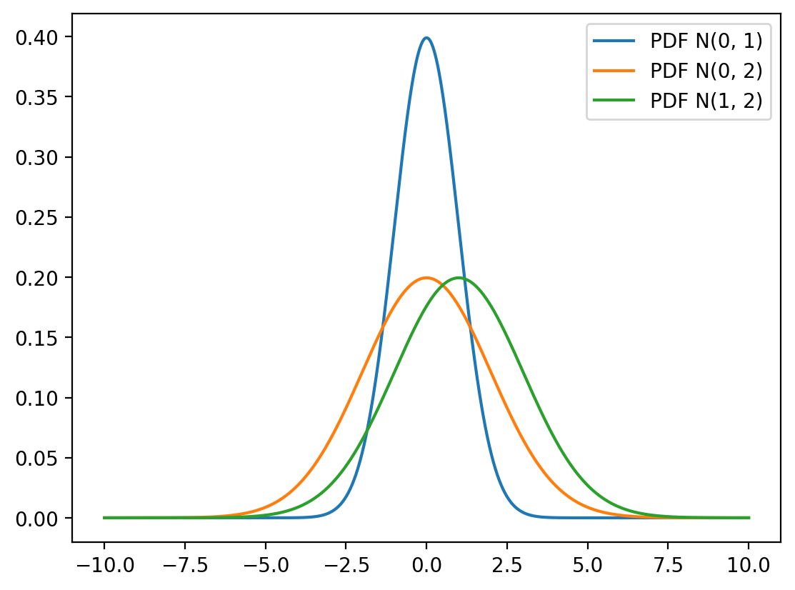
Visualization of Different Parameters
PDF of Normal Distribution
Let \(X\) be a random variable that follows a normal distribution with mean \(\mu\) and variance \(\sigma^2\). The probability density function (PDF) of \(X\) is given by:
\[ f_X(x) = \frac{1}{\sqrt{2\pi\sigma^2}} \exp\left(-\frac{(x-\mu)^2}{2\sigma^2}\right). \]
Let \(X \sim \mathcal{N}(\mu, \sigma^2)\) denote that \(X\) is drawn from a normal distribution with mean \(\mu\) and variance \(\sigma^2\).
Real-World Application: Heights and Weights Data
Human physical measurements often follow normal distributions. Let’s analyze a real dataset of heights and weights:
# Simulating data with normal distributed noise

x_true = torch.linspace(-5, 5, 1000)
y_true = 2 * x_true + 1
eps = torch.distributions.Normal(0, 1).sample(y_true.shape)
y_obs = y_true + eps

plt.scatter(x_true, y_obs,
            label="Observed data",
            marker='o', s=2,
            alpha = 0.5, color='red')
plt.plot(x_true, y_true, label="True data")
plt.legend()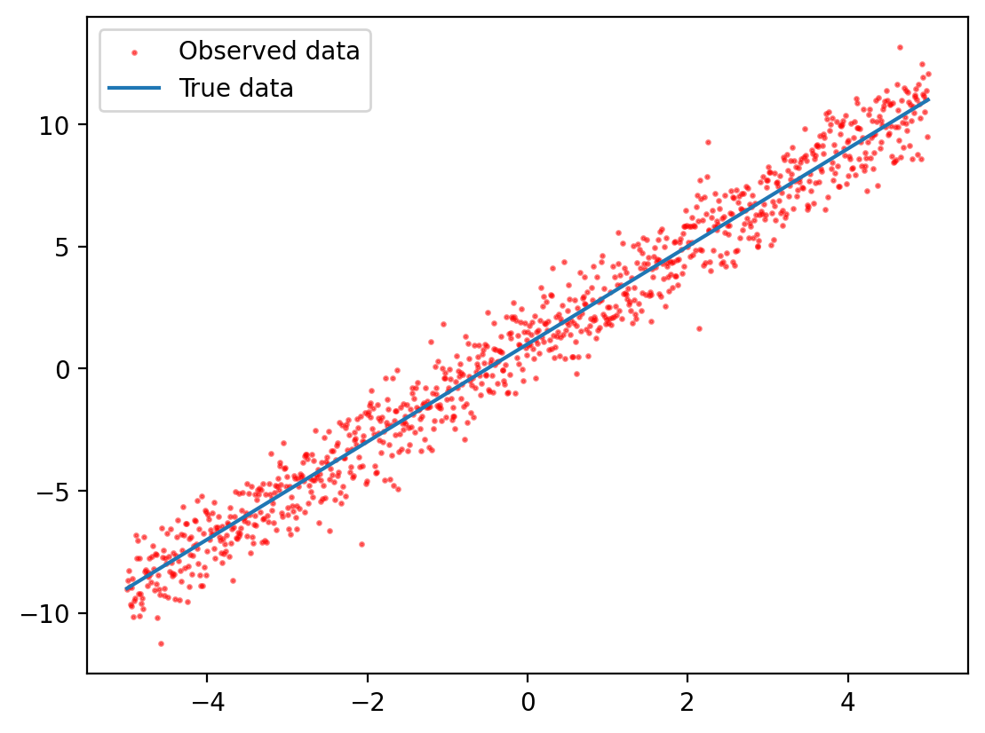
Heights and weights data
The dataset contains 25,000 rows and 3 columns. Each row represents a person and the columns represent the person’s index, height, and weight.
The fitted normal distribution closely matches the empirical height data, confirming that human heights approximately follow a normal distribution.
Weight Distribution Analysis
Let’s examine whether weights also follow a normal distribution:
Practical Application: Grade Distribution
⚠️ Disclaimer: This example is for educational purposes only. I do not endorse using normal distributions for grading in practice, as it can be unfair and arbitrary.
Let’s demonstrate how percentiles work with normal distributions:
| Height(Inches) | Weight(Pounds) | |
|---|---|---|
| 1 | 65.78331 | 112.9925 |
| 2 | 71.51521 | 136.4873 |
| 3 | 69.39874 | 153.0269 |
| 4 | 68.21660 | 142.3354 |
| 5 | 67.78781 | 144.2971 |
fig, ax = plt.subplots(nrows=2, sharex=True)
store_df["Height(Inches)"].plot(kind='density', ax=ax[0])
store_df["Height(Inches)"].plot(kind='hist', bins=30, ax=ax[1])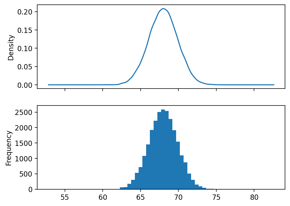
This visualization shows how percentile-based grading works with a normal distribution. Each colored region represents a different grade band based on percentiles.
2. Laplace Distribution
The Laplace distribution is a continuous probability distribution that’s symmetric like the normal distribution but has heavier tails, making it more robust to outliers.
Mathematical Definition
Let \(X \sim \text{Laplace}(\mu, b)\) where \(\mu\) is the location parameter and \(b > 0\) is the scale parameter. The PDF is:
\[f_X(x) = \frac{1}{2b} \exp\left(-\frac{|x-\mu|}{b}\right)\]
Properties
- Mean: \(E[X] = \mu\)
- Variance: \(\text{Var}(X) = 2b^2\)
- Support: \((-\infty, \infty)\)
- Heavier tails than normal distribution
- Used in robust statistics and L1 regularization
Comparison with Normal Distribution
Notice how the Laplace distribution has a sharper peak and heavier tails compared to the normal distribution.
3. Half-Normal Distribution
The Half-Normal distribution is derived from the normal distribution by taking the absolute value, making it useful for modeling positive quantities.
Mathematical Definition
If \(Y \sim \mathcal{N}(0, \sigma^2)\), then \(X = |Y|\) follows a half-normal distribution with PDF:
\[f_X(x) = \sqrt{\frac{2}{\pi\sigma^2}} \exp\left(-\frac{x^2}{2\sigma^2}\right) \quad \text{for } x \geq 0\]
Properties
- Mean: \(E[X] = \sigma\sqrt{\frac{2}{\pi}}\)
- Variance: \(\text{Var}(X) = \sigma^2\left(1-\frac{2}{\pi}\right)\)
- Support: \([0, \infty)\)
- Applications: Error magnitudes, positive measurements
Visualization
# Fit a normal distribution to the data
mu = store_df["Height(Inches)"].mean().item()
sigma = store_df["Height(Inches)"].std().item()

dist = torch.distributions.Normal(mu, sigma)
x = torch.linspace(50, 80, 1000)
y = dist.log_prob(x).exp()
plt.plot(x, y, label="Fitted PDF")

store_df["Height(Inches)"].plot(kind='hist', label="Histogram", density=True, bins=30)
plt.legend()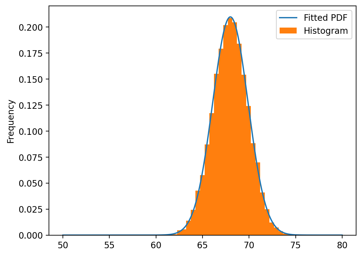
Understanding Log vs Linear Scale
When working with very small probabilities, it’s often useful to work in log space to avoid numerical underflow:
Grading
Note: I DO NOT FOLLOW or endorse using a normal distribution to model grades in a class. This is just an exercise to practice the PDF of a normal distribution and show how to use percentiles.
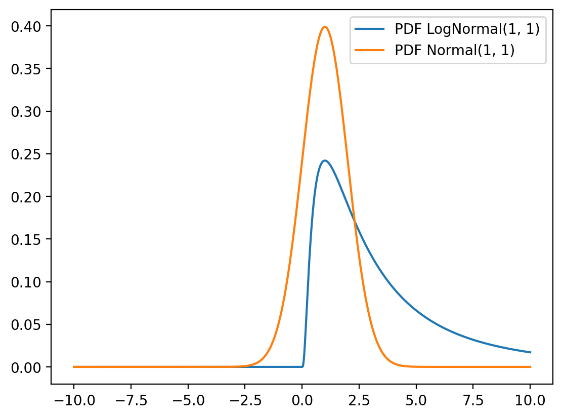
4. Log-Normal Distribution
The Log-Normal distribution arises when the logarithm of a random variable follows a normal distribution. It’s crucial for modeling positive quantities that result from multiplicative processes.
Mathematical Definition
If \(Y \sim \mathcal{N}(\mu, \sigma^2)\), then \(X = e^Y\) follows a log-normal distribution with PDF:
\[f_X(x) = \frac{1}{x\sqrt{2\pi\sigma^2}} \exp\left(-\frac{(\ln(x)-\mu)^2}{2\sigma^2}\right) \quad \text{for } x > 0\]
Properties
- Mean: \(E[X] = e^{\mu + \sigma^2/2}\)
- Variance: \(\text{Var}(X) = e^{2\mu + \sigma^2}(e^{\sigma^2} - 1)\)
- Support: \((0, \infty)\)
- Right-skewed: Always positively skewed
Applications
- Stock prices and financial returns
- File sizes and internet traffic
- Income distributions
- Product lifetimes
- Particle sizes
Comparing Log-Normal with Normal
mu_marks, sigma_marks = marks.mean().item(), marks.std().item()
dist = torch.distributions.Normal(mu_marks, sigma_marks)
x = torch.linspace(30, 110, 1000)
y = dist.log_prob(x).exp()
plt.plot(x, y, label="Fitted PDF", color='gray', lw=2)

# 99% percentile and above get A+
marks_99_per = dist.icdf(torch.tensor(0.99))
num_students_getting_A_plus = marks[marks>marks_99_per].shape[0]
plt.fill_between(x, y, where=x>marks_99_per, alpha=0.5, label=f"A+ ({num_students_getting_A_plus})")

# 90th percntile to 99th percentile get A
marks_90_per = dist.icdf(torch.tensor(0.90))
num_students_getting_A = marks[(marks>marks_90_per) & (marks<marks_99_per)].shape[0]
plt.fill_between(x, y, where=(x>marks_90_per) & (x<marks_99_per), alpha=0.5, label=f"A ({num_students_getting_A})")

# 75th percentile to 90th percentile get A-
marks_75_per = dist.icdf(torch.tensor(0.75))
num_students_getting_B = marks[(marks>marks_75_per) & (marks<marks_90_per)].shape[0]
plt.fill_between(x, y, where=(x>marks_75_per) & (x<marks_90_per), alpha=0.5, label=f"B ({num_students_getting_B})")

# 60th percentile to 75th percentile get B
marks_60_per = dist.icdf(torch.tensor(0.60))
num_students_getting_B = marks[(marks>marks_60_per) & (marks<marks_75_per)].shape[0]
plt.fill_between(x, y, where=(x>marks_60_per) & (x<marks_75_per), alpha=0.5, label=f"B- ({num_students_getting_B})")

# 45th percentile to 60th percentile get C
marks_45_per = dist.icdf(torch.tensor(0.45))
num_students_getting_B_minus = marks[(marks>marks_45_per) & (marks<marks_60_per)].shape[0]
plt.fill_between(x, y, where=(x>marks_45_per) & (x<marks_60_per), alpha=0.5, label=f"C ({num_students_getting_B_minus})")

#35th percentile to 45th percentile get C-
marks_35_per = dist.icdf(torch.tensor(0.35))
num_students_getting_C = marks[(marks>marks_35_per) & (marks<marks_45_per)].shape[0]
plt.fill_between(x, y, where=(x>marks_35_per) & (x<marks_45_per), alpha=0.5, label=f"C- ({num_students_getting_C})")

# 20th percentile to 35th percentile get D
marks_20_per = dist.icdf(torch.tensor(0.20))
num_students_getting_C_minus = marks[(marks>marks_20_per) & (marks<marks_35_per)].shape[0]
plt.fill_between(x, y, where=(x>marks_20_per) & (x<marks_35_per), alpha=0.5, label=f"D ({num_students_getting_C_minus})")

# 3rd percentile to 20th percentile get E
marks_3_per = dist.icdf(torch.tensor(0.03))
num_students_getting_D = marks[(marks>marks_3_per) & (marks<marks_20_per)].shape[0]
plt.fill_between(x, y, where=(x>marks_3_per) & (x<marks_20_per), alpha=0.5, label=f"E ({num_students_getting_D})")

# 3rd percentile and below get F
num_students_getting_F = marks[marks<marks_3_per].shape[0]
plt.fill_between(x, y, where=x<marks_3_per, alpha=0.5, label=f"F ({num_students_getting_F})")

plt.legend()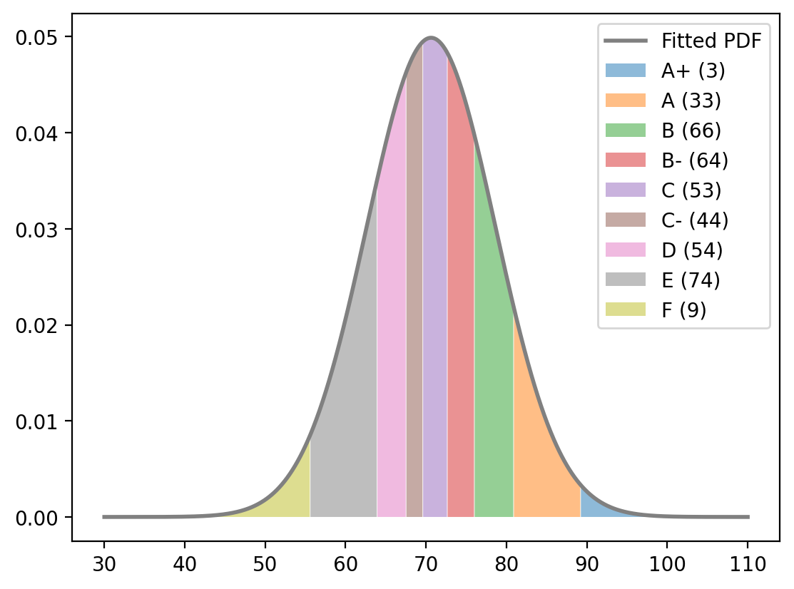
Laplace Distribution
Let \(X\) be a random variable that follows a Laplace distribution with mean \(\mu\) and scale \(\lambda\). The probability density function (PDF) of \(X\) is given by:
\[ f_X(x) = \frac{1}{2\lambda} \exp\left(-\frac{|x-\mu|}{\lambda}\right). \]
unit_normal = torch.distributions.Normal(0, 1)
unit_laplace = torch.distributions.Laplace(0, 1)

x = torch.linspace(-10, 10, 1000)
y_normal = unit_normal.log_prob(x).exp()
y_laplace = unit_laplace.log_prob(x).exp()
plt.plot(x, y_normal, label="Normal")
plt.plot(x, y_laplace, label="Laplace")
plt.legend()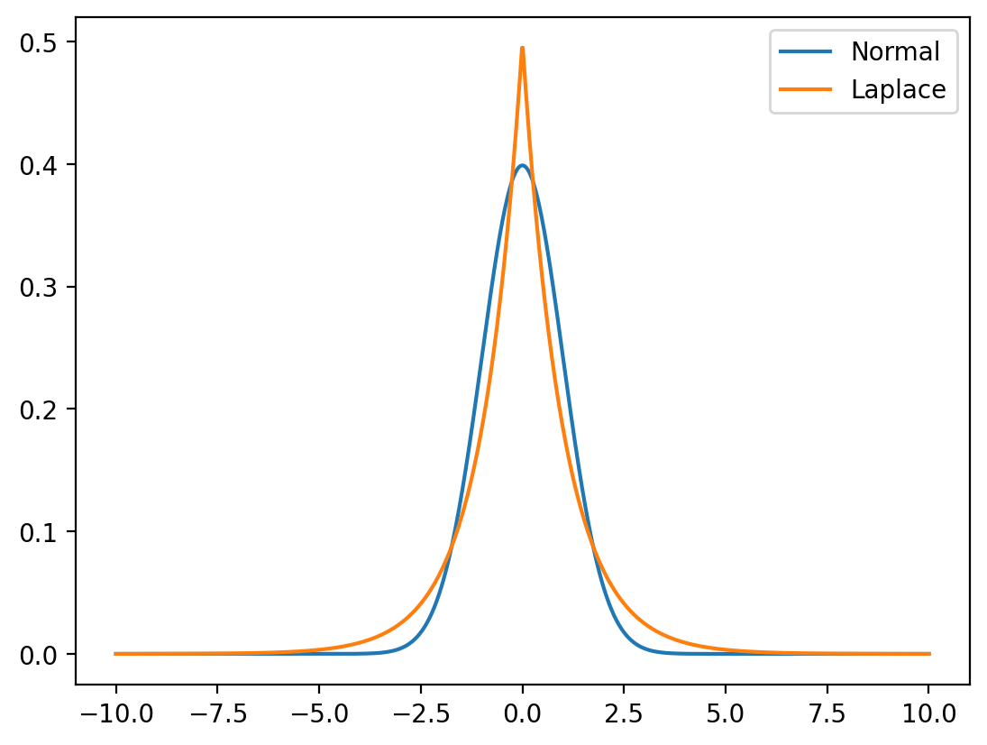
Real-World Example: Chess Game Lengths
Let’s analyze whether chess game lengths follow a log-normal distribution:
Half Normal Distribution
Let \(Y\) follow the normal distribution with mean \(0\) and variance \(\sigma^2\). The half normal distribution is obtained by taking the absolute value of \(Y\). \(X = |Y|\) follows a half normal distribution with mean \(\sqrt{\frac{2}{\pi}}\sigma\) and variance \(\sigma^2(1-\frac{2}{\pi})\).
The probability density function (PDF) of \(X\) is given by:
$$ f_X(x) = (-).
$$
hn = torch.distributions.HalfNormal(1)
x = torch.linspace(-10, 10, 1000)
try:
    y = hn.log_prob(x).exp()
    plt.plot(x, y, label="HalfNormal")
except Exception as e:
    print(e)
Expected value argument (Tensor of shape (1000,)) to be within the support (GreaterThanEq(lower_bound=0.0)) of the distribution HalfNormal(), but found invalid values:
tensor([-10.0000, -9.9800, -9.9600, -9.9399, -9.9199, -9.8999, -9.8799,
-9.8599, -9.8398, -9.8198, -9.7998, -9.7798, -9.7598, -9.7397,
-9.7197, -9.6997, -9.6797, -9.6597, -9.6396, -9.6196, -9.5996,
-9.5796, -9.5596, -9.5395, -9.5195, -9.4995, -9.4795, -9.4595,
-9.4394, -9.4194, -9.3994, -9.3794, -9.3594, -9.3393, -9.3193,
-9.2993, -9.2793, -9.2593, -9.2392, -9.2192, -9.1992, -9.1792,
-9.1592, -9.1391, -9.1191, -9.0991, -9.0791, -9.0591, -9.0390,
-9.0190, -8.9990, -8.9790, -8.9590, -8.9389, -8.9189, -8.8989,
-8.8789, -8.8589, -8.8388, -8.8188, -8.7988, -8.7788, -8.7588,
-8.7387, -8.7187, -8.6987, -8.6787, -8.6587, -8.6386, -8.6186,
-8.5986, -8.5786, -8.5586, -8.5385, -8.5185, -8.4985, -8.4785,
-8.4585, -8.4384, -8.4184, -8.3984, -8.3784, -8.3584, -8.3383,
-8.3183, -8.2983, -8.2783, -8.2583, -8.2382, -8.2182, -8.1982,
-8.1782, -8.1582, -8.1381, -8.1181, -8.0981, -8.0781, -8.0581,
-8.0380, -8.0180, -7.9980, -7.9780, -7.9580, -7.9379, -7.9179,
-7.8979, -7.8779, -7.8579, -7.8378, -7.8178, -7.7978, -7.7778,
-7.7578, -7.7377, -7.7177, -7.6977, -7.6777, -7.6577, -7.6376,
-7.6176, -7.5976, -7.5776, -7.5576, -7.5375, -7.5175, -7.4975,
-7.4775, -7.4575, -7.4374, -7.4174, -7.3974, -7.3774, -7.3574,
-7.3373, -7.3173, -7.2973, -7.2773, -7.2573, -7.2372, -7.2172,
-7.1972, -7.1772, -7.1572, -7.1371, -7.1171, -7.0971, -7.0771,
-7.0571, -7.0370, -7.0170, -6.9970, -6.9770, -6.9570, -6.9369,
-6.9169, -6.8969, -6.8769, -6.8569, -6.8368, -6.8168, -6.7968,
-6.7768, -6.7568, -6.7367, -6.7167, -6.6967, -6.6767, -6.6567,
-6.6366, -6.6166, -6.5966, -6.5766, -6.5566, -6.5365, -6.5165,
-6.4965, -6.4765, -6.4565, -6.4364, -6.4164, -6.3964, -6.3764,
-6.3564, -6.3363, -6.3163, -6.2963, -6.2763, -6.2563, -6.2362,
-6.2162, -6.1962, -6.1762, -6.1562, -6.1361, -6.1161, -6.0961,
-6.0761, -6.0561, -6.0360, -6.0160, -5.9960, -5.9760, -5.9560,
-5.9359, -5.9159, -5.8959, -5.8759, -5.8559, -5.8358, -5.8158,
-5.7958, -5.7758, -5.7558, -5.7357, -5.7157, -5.6957, -5.6757,
-5.6557, -5.6356, -5.6156, -5.5956, -5.5756, -5.5556, -5.5355,
-5.5155, -5.4955, -5.4755, -5.4555, -5.4354, -5.4154, -5.3954,
-5.3754, -5.3554, -5.3353, -5.3153, -5.2953, -5.2753, -5.2553,
-5.2352, -5.2152, -5.1952, -5.1752, -5.1552, -5.1351, -5.1151,
-5.0951, -5.0751, -5.0551, -5.0350, -5.0150, -4.9950, -4.9750,
-4.9550, -4.9349, -4.9149, -4.8949, -4.8749, -4.8549, -4.8348,
-4.8148, -4.7948, -4.7748, -4.7548, -4.7347, -4.7147, -4.6947,
-4.6747, -4.6547, -4.6346, -4.6146, -4.5946, -4.5746, -4.5546,
-4.5345, -4.5145, -4.4945, -4.4745, -4.4545, -4.4344, -4.4144,
-4.3944, -4.3744, -4.3544, -4.3343, -4.3143, -4.2943, -4.2743,
-4.2543, -4.2342, -4.2142, -4.1942, -4.1742, -4.1542, -4.1341,
-4.1141, -4.0941, -4.0741, -4.0541, -4.0340, -4.0140, -3.9940,
-3.9740, -3.9540, -3.9339, -3.9139, -3.8939, -3.8739, -3.8539,
-3.8338, -3.8138, -3.7938, -3.7738, -3.7538, -3.7337, -3.7137,
-3.6937, -3.6737, -3.6537, -3.6336, -3.6136, -3.5936, -3.5736,
-3.5536, -3.5335, -3.5135, -3.4935, -3.4735, -3.4535, -3.4334,
-3.4134, -3.3934, -3.3734, -3.3534, -3.3333, -3.3133, -3.2933,
-3.2733, -3.2533, -3.2332, -3.2132, -3.1932, -3.1732, -3.1532,
-3.1331, -3.1131, -3.0931, -3.0731, -3.0531, -3.0330, -3.0130,
-2.9930, -2.9730, -2.9530, -2.9329, -2.9129, -2.8929, -2.8729,
-2.8529, -2.8328, -2.8128, -2.7928, -2.7728, -2.7528, -2.7327,
-2.7127, -2.6927, -2.6727, -2.6527, -2.6326, -2.6126, -2.5926,
-2.5726, -2.5526, -2.5325, -2.5125, -2.4925, -2.4725, -2.4525,
-2.4324, -2.4124, -2.3924, -2.3724, -2.3524, -2.3323, -2.3123,
-2.2923, -2.2723, -2.2523, -2.2322, -2.2122, -2.1922, -2.1722,
-2.1522, -2.1321, -2.1121, -2.0921, -2.0721, -2.0521, -2.0320,
-2.0120, -1.9920, -1.9720, -1.9520, -1.9319, -1.9119, -1.8919,
-1.8719, -1.8519, -1.8318, -1.8118, -1.7918, -1.7718, -1.7518,
-1.7317, -1.7117, -1.6917, -1.6717, -1.6517, -1.6316, -1.6116,
-1.5916, -1.5716, -1.5516, -1.5315, -1.5115, -1.4915, -1.4715,
-1.4515, -1.4314, -1.4114, -1.3914, -1.3714, -1.3514, -1.3313,
-1.3113, -1.2913, -1.2713, -1.2513, -1.2312, -1.2112, -1.1912,
-1.1712, -1.1512, -1.1311, -1.1111, -1.0911, -1.0711, -1.0511,
-1.0310, -1.0110, -0.9910, -0.9710, -0.9510, -0.9309, -0.9109,
-0.8909, -0.8709, -0.8509, -0.8308, -0.8108, -0.7908, -0.7708,
-0.7508, -0.7307, -0.7107, -0.6907, -0.6707, -0.6507, -0.6306,
-0.6106, -0.5906, -0.5706, -0.5506, -0.5305, -0.5105, -0.4905,
-0.4705, -0.4505, -0.4304, -0.4104, -0.3904, -0.3704, -0.3504,
-0.3303, -0.3103, -0.2903, -0.2703, -0.2503, -0.2302, -0.2102,
-0.1902, -0.1702, -0.1502, -0.1301, -0.1101, -0.0901, -0.0701,
-0.0501, -0.0300, -0.0100, 0.0100, 0.0300, 0.0500, 0.0701,
0.0901, 0.1101, 0.1301, 0.1502, 0.1702, 0.1902, 0.2102,
0.2302, 0.2503, 0.2703, 0.2903, 0.3103, 0.3303, 0.3504,
0.3704, 0.3904, 0.4104, 0.4304, 0.4505, 0.4705, 0.4905,
0.5105, 0.5305, 0.5506, 0.5706, 0.5906, 0.6106, 0.6306,
0.6507, 0.6707, 0.6907, 0.7107, 0.7307, 0.7508, 0.7708,
0.7908, 0.8108, 0.8308, 0.8509, 0.8709, 0.8909, 0.9109,
0.9309, 0.9510, 0.9710, 0.9910, 1.0110, 1.0310, 1.0511,
1.0711, 1.0911, 1.1111, 1.1311, 1.1512, 1.1712, 1.1912,
1.2112, 1.2312, 1.2513, 1.2713, 1.2913, 1.3113, 1.3313,
1.3514, 1.3714, 1.3914, 1.4114, 1.4314, 1.4515, 1.4715,
1.4915, 1.5115, 1.5315, 1.5516, 1.5716, 1.5916, 1.6116,
1.6316, 1.6517, 1.6717, 1.6917, 1.7117, 1.7317, 1.7518,
1.7718, 1.7918, 1.8118, 1.8318, 1.8519, 1.8719, 1.8919,
1.9119, 1.9319, 1.9520, 1.9720, 1.9920, 2.0120, 2.0320,
2.0521, 2.0721, 2.0921, 2.1121, 2.1321, 2.1522, 2.1722,
2.1922, 2.2122, 2.2322, 2.2523, 2.2723, 2.2923, 2.3123,
2.3323, 2.3524, 2.3724, 2.3924, 2.4124, 2.4324, 2.4525,
2.4725, 2.4925, 2.5125, 2.5325, 2.5526, 2.5726, 2.5926,
2.6126, 2.6326, 2.6527, 2.6727, 2.6927, 2.7127, 2.7327,
2.7528, 2.7728, 2.7928, 2.8128, 2.8328, 2.8529, 2.8729,
2.8929, 2.9129, 2.9329, 2.9530, 2.9730, 2.9930, 3.0130,
3.0330, 3.0531, 3.0731, 3.0931, 3.1131, 3.1331, 3.1532,
3.1732, 3.1932, 3.2132, 3.2332, 3.2533, 3.2733, 3.2933,
3.3133, 3.3333, 3.3534, 3.3734, 3.3934, 3.4134, 3.4334,
3.4535, 3.4735, 3.4935, 3.5135, 3.5335, 3.5536, 3.5736,
3.5936, 3.6136, 3.6336, 3.6537, 3.6737, 3.6937, 3.7137,
3.7337, 3.7538, 3.7738, 3.7938, 3.8138, 3.8338, 3.8539,
3.8739, 3.8939, 3.9139, 3.9339, 3.9540, 3.9740, 3.9940,
4.0140, 4.0340, 4.0541, 4.0741, 4.0941, 4.1141, 4.1341,
4.1542, 4.1742, 4.1942, 4.2142, 4.2342, 4.2543, 4.2743,
4.2943, 4.3143, 4.3343, 4.3544, 4.3744, 4.3944, 4.4144,
4.4344, 4.4545, 4.4745, 4.4945, 4.5145, 4.5345, 4.5546,
4.5746, 4.5946, 4.6146, 4.6346, 4.6547, 4.6747, 4.6947,
4.7147, 4.7347, 4.7548, 4.7748, 4.7948, 4.8148, 4.8348,
4.8549, 4.8749, 4.8949, 4.9149, 4.9349, 4.9550, 4.9750,
4.9950, 5.0150, 5.0350, 5.0551, 5.0751, 5.0951, 5.1151,
5.1351, 5.1552, 5.1752, 5.1952, 5.2152, 5.2352, 5.2553,
5.2753, 5.2953, 5.3153, 5.3353, 5.3554, 5.3754, 5.3954,
5.4154, 5.4354, 5.4555, 5.4755, 5.4955, 5.5155, 5.5355,
5.5556, 5.5756, 5.5956, 5.6156, 5.6356, 5.6557, 5.6757,
5.6957, 5.7157, 5.7357, 5.7558, 5.7758, 5.7958, 5.8158,
5.8358, 5.8559, 5.8759, 5.8959, 5.9159, 5.9359, 5.9560,
5.9760, 5.9960, 6.0160, 6.0360, 6.0561, 6.0761, 6.0961,
6.1161, 6.1361, 6.1562, 6.1762, 6.1962, 6.2162, 6.2362,
6.2563, 6.2763, 6.2963, 6.3163, 6.3363, 6.3564, 6.3764,
6.3964, 6.4164, 6.4364, 6.4565, 6.4765, 6.4965, 6.5165,
6.5365, 6.5566, 6.5766, 6.5966, 6.6166, 6.6366, 6.6567,
6.6767, 6.6967, 6.7167, 6.7367, 6.7568, 6.7768, 6.7968,
6.8168, 6.8368, 6.8569, 6.8769, 6.8969, 6.9169, 6.9369,
6.9570, 6.9770, 6.9970, 7.0170, 7.0370, 7.0571, 7.0771,
7.0971, 7.1171, 7.1371, 7.1572, 7.1772, 7.1972, 7.2172,
7.2372, 7.2573, 7.2773, 7.2973, 7.3173, 7.3373, 7.3574,
7.3774, 7.3974, 7.4174, 7.4374, 7.4575, 7.4775, 7.4975,
7.5175, 7.5375, 7.5576, 7.5776, 7.5976, 7.6176, 7.6376,
7.6577, 7.6777, 7.6977, 7.7177, 7.7377, 7.7578, 7.7778,
7.7978, 7.8178, 7.8378, 7.8579, 7.8779, 7.8979, 7.9179,
7.9379, 7.9580, 7.9780, 7.9980, 8.0180, 8.0380, 8.0581,
8.0781, 8.0981, 8.1181, 8.1381, 8.1582, 8.1782, 8.1982,
8.2182, 8.2382, 8.2583, 8.2783, 8.2983, 8.3183, 8.3383,
8.3584, 8.3784, 8.3984, 8.4184, 8.4384, 8.4585, 8.4785,
8.4985, 8.5185, 8.5385, 8.5586, 8.5786, 8.5986, 8.6186,
8.6386, 8.6587, 8.6787, 8.6987, 8.7187, 8.7387, 8.7588,
8.7788, 8.7988, 8.8188, 8.8388, 8.8589, 8.8789, 8.8989,
8.9189, 8.9389, 8.9590, 8.9790, 8.9990, 9.0190, 9.0390,
9.0591, 9.0791, 9.0991, 9.1191, 9.1391, 9.1592, 9.1792,
9.1992, 9.2192, 9.2392, 9.2593, 9.2793, 9.2993, 9.3193,
9.3393, 9.3594, 9.3794, 9.3994, 9.4194, 9.4394, 9.4595,
9.4795, 9.4995, 9.5195, 9.5395, 9.5596, 9.5796, 9.5996,
9.6196, 9.6396, 9.6597, 9.6797, 9.6997, 9.7197, 9.7397,
9.7598, 9.7798, 9.7998, 9.8198, 9.8398, 9.8599, 9.8799,
9.8999, 9.9199, 9.9399, 9.9600, 9.9800, 10.0000])hn = torch.distributions.HalfNormal(1)
x = torch.linspace(-10, 10, 1000)
x_mask = x>0
y = torch.zeros_like(x)
y[x_mask] = hn.log_prob(x[x_mask]).exp()
plt.plot(x, y, label="Half Normal")
normal = torch.distributions.Normal(0, 1)
y_norm = normal.log_prob(x).exp()
plt.plot(x, y_norm, label="Normal")
plt.legend()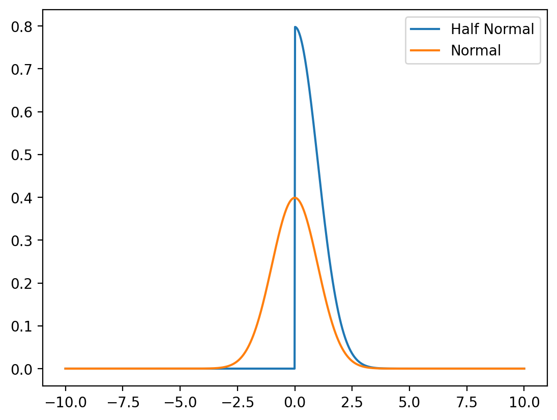
dist = torch.distributions.Normal(0, 1)
x_lin = torch.linspace(-17, 17, 1000)
log_probs = dist.log_prob(x_lin)
probs = log_probs.exp()

fig, ax = plt.subplots(nrows=2, sharex=True)
ax[0].plot(x_lin, log_probs)
ax[0].set_title("Log Prob")
ax[1].plot(x_lin, probs)
ax[1].set_title("Prob")
Text(0.5, 1.0, 'Prob')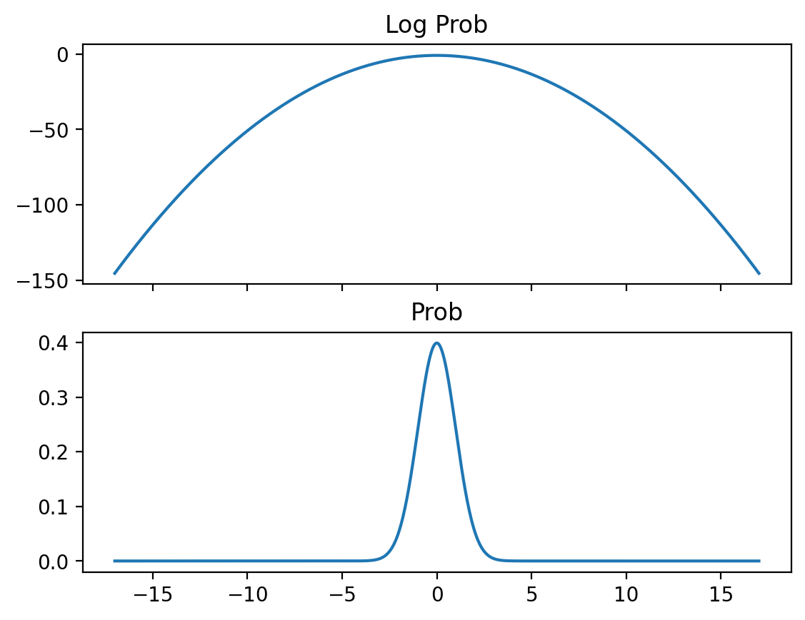
tensor(0.) tensor(0.)
tensor(-145.4189) tensor(-144.8409)
Log Normal Distribution
Let \(Y \sim \mathcal{N}(\mu, \sigma^2)\) be a normally distributed random variable.
Let us define a new random variable \(X = \exp(Y)\).
We can say that log of \(X\) is normally distributed, i.e., \(\log(X) \sim \mathcal{N}(\mu, \sigma^2)\).
We can also say that \(X\) is log-normally distributed.
The probability density function (PDF) of \(X\) is given by:
\[ f_X(x) = \frac{1}{x\sqrt{2\pi\sigma^2}} \exp\left(-\frac{(\log(x)-\mu)^2}{2\sigma^2}\right). \]
We can derive the PDF of \(X\) using the change of variables formula. (will be covered later in the course)
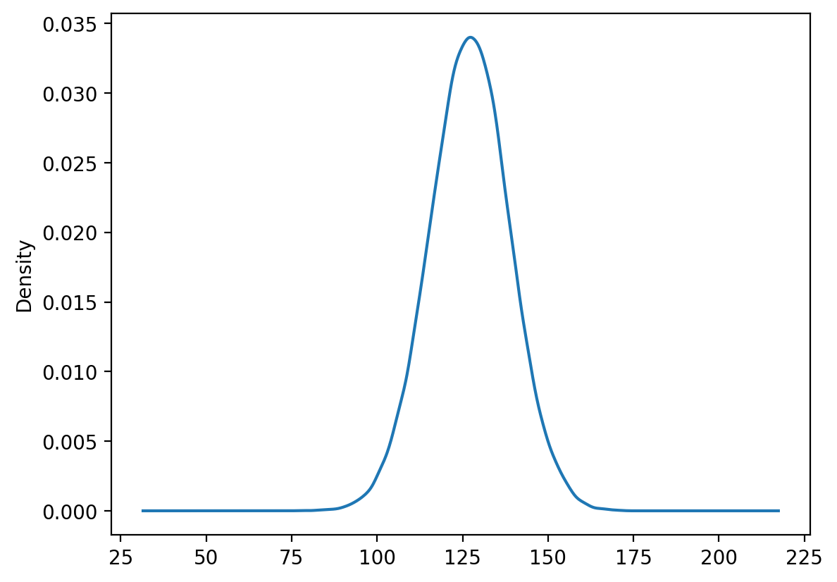
The log-normal distribution provides a reasonable fit to the chess game length data, supporting the hypothesis that game lengths follow a log-normal distribution.
5. Gamma Distribution
The Gamma distribution is a versatile continuous distribution that generalizes the exponential distribution and is widely used for modeling waiting times and positive-valued data.
Mathematical Definition
Let \(X \sim \text{Gamma}(\alpha, \beta)\) where \(\alpha > 0\) is the shape parameter and \(\beta > 0\) is the rate parameter. The PDF is:
\[f_X(x) = \frac{\beta^\alpha}{\Gamma(\alpha)} x^{\alpha-1} e^{-\beta x} \quad \text{for } x > 0\]
where \(\Gamma(\alpha) = \int_0^\infty t^{\alpha-1} e^{-t} dt\) is the gamma function.
Properties
- Mean: \(E[X] = \frac{\alpha}{\beta}\)
- Variance: \(\text{Var}(X) = \frac{\alpha}{\beta^2}\)
- Support: \((0, \infty)\)
- Special cases: Exponential(\(\lambda\)) = Gamma(1, \(\lambda\))
Applications
- Waiting times for multiple events
- Insurance claims modeling
- Rainfall amounts
- Queue lengths
- Reliability engineering
Parameter Estimation Example
Let’s fit a gamma distribution to chess game length data:
6. Uniform Distribution
The Uniform distribution assigns equal probability density to all values within a specified interval, making it fundamental for random number generation and modeling complete uncertainty.
Mathematical Definition
Let \(X \sim \text{Uniform}(a, b)\) where \(a < b\). The PDF is:
\[f_X(x) = \begin{cases} \frac{1}{b-a} & \text{if } a \leq x \leq b \\ 0 & \text{otherwise} \end{cases}\]
Properties
- Mean: \(E[X] = \frac{a+b}{2}\)
- Variance: \(\text{Var}(X) = \frac{(b-a)^2}{12}\)
- Support: \([a, b]\)
- Maximum entropy among distributions with bounded support
Applications
- Random number generation
- Monte Carlo simulations
- Modeling complete uncertainty
- Quality control (tolerance intervals)
- Signal processing (quantization error)
Practical Application: Quantization Error Modeling
Digital signal processing often involves quantizing continuous signals into discrete levels, introducing quantization error that can be modeled as uniform:
x = torch.linspace(-10, 10, 1000)
x_non_neg_mask = x > 0.001

y = torch.zeros_like(x)
y[x_non_neg_mask] = log_normal.log_prob(x[x_non_neg_mask]).exp()
plt.plot(x, y, label="PDF LogNormal(1, 1)")

normal = torch.distributions.Normal(mu, sigma)
plt.plot(x, normal.log_prob(x).exp(), label="PDF Normal(1, 1)")

plt.legend()
Applications
See: https://en.wikipedia.org/wiki/Log-normal_distribution
See https://chess.stackexchange.com/questions/2506/what-is-the-average-length-of-a-game-of-chess/4899#4899
import kagglehub

# Download latest version
path = kagglehub.dataset_download("datasnaek/chess")

print("Path to dataset files:", path)
Path to dataset files: /Users/nipun/.cache/kagglehub/datasets/datasnaek/chess/versions/1| id | rated | created_at | last_move_at | turns | victory_status | winner | increment_code | white_id | white_rating | black_id | black_rating | moves | opening_eco | opening_name | opening_ply | |
|---|---|---|---|---|---|---|---|---|---|---|---|---|---|---|---|---|
| 0 | TZJHLljE | False | 1.504210e+12 | 1.504210e+12 | 13 | outoftime | white | 15+2 | bourgris | 1500 | a-00 | 1191 | d4 d5 c4 c6 cxd5 e6 dxe6 fxe6 Nf3 Bb4+ Nc3 Ba5... | D10 | Slav Defense: Exchange Variation | 5 |
| 1 | l1NXvwaE | True | 1.504130e+12 | 1.504130e+12 | 16 | resign | black | 5+10 | a-00 | 1322 | skinnerua | 1261 | d4 Nc6 e4 e5 f4 f6 dxe5 fxe5 fxe5 Nxe5 Qd4 Nc6... | B00 | Nimzowitsch Defense: Kennedy Variation | 4 |
| 2 | mIICvQHh | True | 1.504130e+12 | 1.504130e+12 | 61 | mate | white | 5+10 | ischia | 1496 | a-00 | 1500 | e4 e5 d3 d6 Be3 c6 Be2 b5 Nd2 a5 a4 c5 axb5 Nc... | C20 | King's Pawn Game: Leonardis Variation | 3 |
| 3 | kWKvrqYL | True | 1.504110e+12 | 1.504110e+12 | 61 | mate | white | 20+0 | daniamurashov | 1439 | adivanov2009 | 1454 | d4 d5 Nf3 Bf5 Nc3 Nf6 Bf4 Ng4 e3 Nc6 Be2 Qd7 O... | D02 | Queen's Pawn Game: Zukertort Variation | 3 |
| 4 | 9tXo1AUZ | True | 1.504030e+12 | 1.504030e+12 | 95 | mate | white | 30+3 | nik221107 | 1523 | adivanov2009 | 1469 | e4 e5 Nf3 d6 d4 Nc6 d5 Nb4 a3 Na6 Nc3 Be7 b4 N... | C41 | Philidor Defense | 5 |
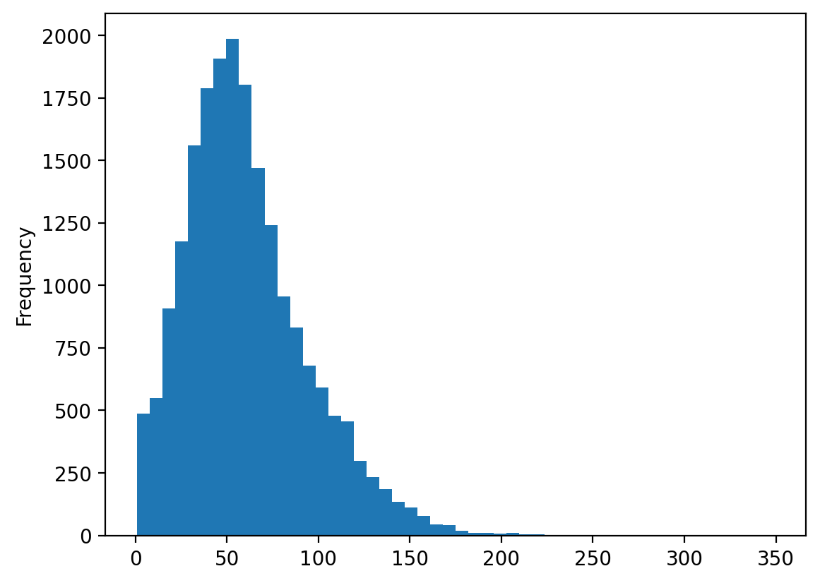
# Logarithm of the number of turns
df["turns"].apply(np.log).plot(kind='hist', bins=50)

# Log of turns seems to be normally distributed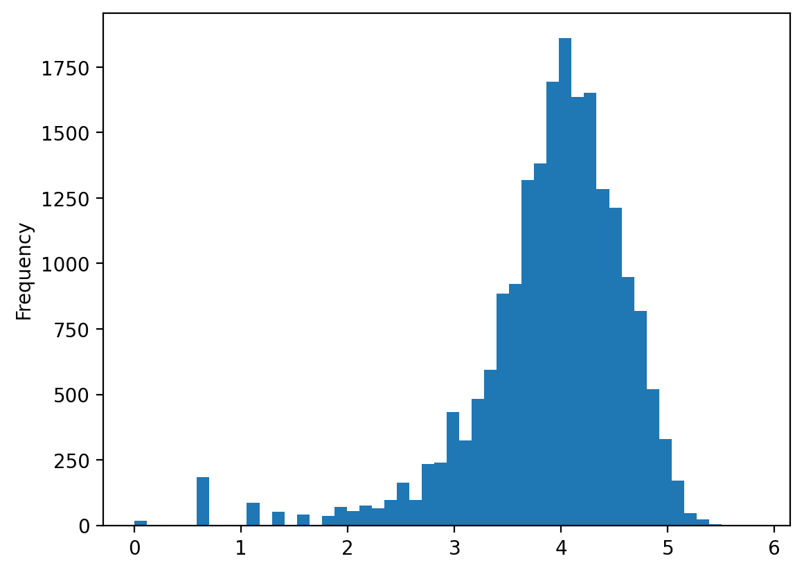
3.9070571274448245 0.6822030192719669# Plot PDF of the fitted log-normal distribution
x = torch.linspace(0.001, 300, 1000)
with torch.no_grad():
log_normal = torch.distributions.LogNormal(mu, sigma)
y = log_normal.log_prob(x).exp()
plt.plot(x, y, label="Fitted PDF")
plt.hist(df["turns"], bins=50, density=True, alpha=0.5, label="KDE")
plt.legend()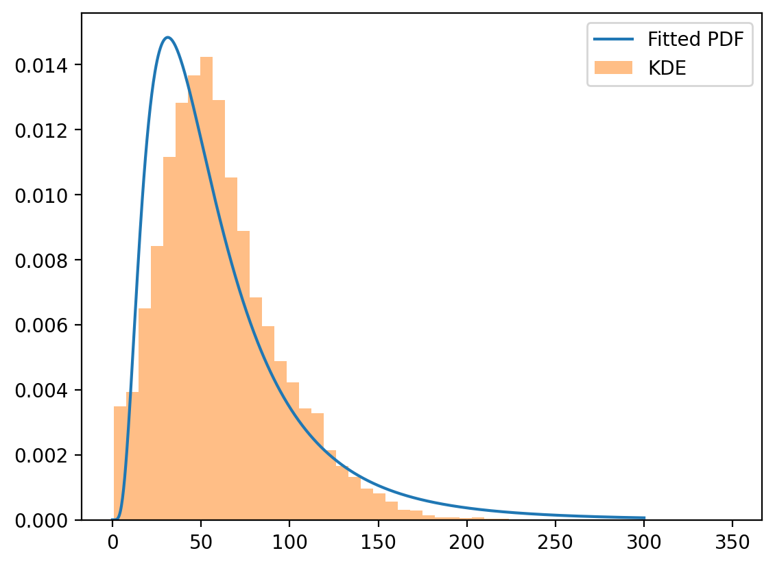
Gamma distribution
Let \(X\) be a random variable that follows a gamma distribution with shape parameter \(k\) and scale parameter \(\theta\). The probability density function (PDF) of \(X\) is given by:
\[ f_X(x) = \frac{1}{\Gamma(k)\theta^k} x^{k-1} \exp\left(-\frac{x}{\theta}\right). \]
where \(\Gamma(k)\) is the gamma function defined as:
\[ \Gamma(k) = \int_0^\infty x^{k-1} e^{-x} dx. \]
The quantization error closely follows the theoretical uniform distribution, validating our modeling approach.
Audio Compression Example
Let’s demonstrate quantization with real audio data:
gamma_dist = torch.distributions.Gamma(2, 1)

x = torch.linspace(0.001, 10, 1000)
y = gamma_dist.log_prob(x).exp()
plt.plot(x, y, label="PDF Gamma(2, 1)")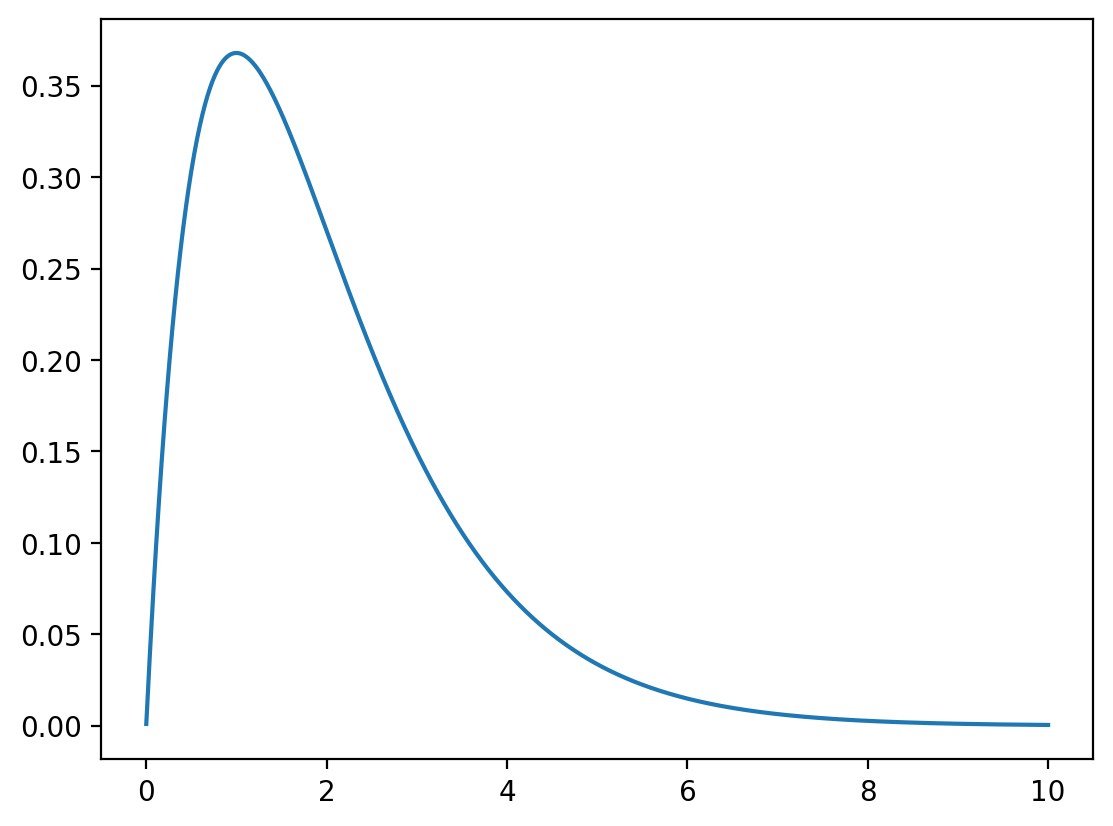
# Fit a gamma distribution to the data
alpha, beta = torch.tensor([1.0], requires_grad=True), torch.tensor([1.0], requires_grad=True)
gamma_dist = torch.distributions.Gamma(alpha, beta)

optimizer = torch.optim.Adam([alpha, beta], lr=0.01)

x = torch.tensor(df["turns"].values, dtype=torch.float32)

for i in range(1000):
    optimizer.zero_grad()
    loss = -gamma_dist.log_prob(x).mean()
    loss.backward()
    optimizer.step()

print(alpha.item(), beta.item())
2.315873384475708 0.03829348832368851
Uniform Distribution
Let \(X\) be a random variable that follows a uniform distribution on the interval \([a, b]\). The probability density function (PDF) of \(X\) is given by:
$$ f_X(x) = \[\begin{cases} \frac{1}{b-a} & \text{if } x \in [a, b], \\ 0 & \text{otherwise}. \end{cases}\]$$
We can say that \(X \sim \text{Uniform}(a, b)\).
7. Beta Distribution
The Beta distribution is defined on the interval [0,1] and is extremely versatile for modeling proportions, probabilities, and bounded quantities.
Mathematical Definition
Let \(X \sim \text{Beta}(\alpha, \beta)\) where \(\alpha, \beta > 0\). The PDF is:
\[f_X(x) = \frac{\Gamma(\alpha + \beta)}{\Gamma(\alpha)\Gamma(\beta)} x^{\alpha-1} (1-x)^{\beta-1} \quad \text{for } 0 < x < 1\]
Properties
- Mean: \(E[X] = \frac{\alpha}{\alpha + \beta}\)
- Variance: \(\text{Var}(X) = \frac{\alpha\beta}{(\alpha + \beta)^2(\alpha + \beta + 1)}\)
- Support: \((0, 1)\)
- Conjugate prior for Bernoulli/Binomial likelihood
Shape Flexibility
The Beta distribution can take many shapes depending on its parameters:
x_range = torch.linspace(-1, 3, 1000)
try:
    y = dist.log_prob(x_range).exp()
except Exception as e:
    print(e)
Expected value argument (Tensor of shape (1000,)) to be within the support (Interval(lower_bound=0.0, upper_bound=2.0)) of the distribution Uniform(low: 0.0, high: 2.0), but found invalid values:
tensor([-1.0000e+00, -9.9600e-01, -9.9199e-01, -9.8799e-01, -9.8398e-01,
-9.7998e-01, -9.7598e-01, -9.7197e-01, -9.6797e-01, -9.6396e-01,
-9.5996e-01, -9.5596e-01, -9.5195e-01, -9.4795e-01, -9.4394e-01,
-9.3994e-01, -9.3594e-01, -9.3193e-01, -9.2793e-01, -9.2392e-01,
-9.1992e-01, -9.1592e-01, -9.1191e-01, -9.0791e-01, -9.0390e-01,
-8.9990e-01, -8.9590e-01, -8.9189e-01, -8.8789e-01, -8.8388e-01,
-8.7988e-01, -8.7588e-01, -8.7187e-01, -8.6787e-01, -8.6386e-01,
-8.5986e-01, -8.5586e-01, -8.5185e-01, -8.4785e-01, -8.4384e-01,
-8.3984e-01, -8.3584e-01, -8.3183e-01, -8.2783e-01, -8.2382e-01,
-8.1982e-01, -8.1582e-01, -8.1181e-01, -8.0781e-01, -8.0380e-01,
-7.9980e-01, -7.9580e-01, -7.9179e-01, -7.8779e-01, -7.8378e-01,
-7.7978e-01, -7.7578e-01, -7.7177e-01, -7.6777e-01, -7.6376e-01,
-7.5976e-01, -7.5576e-01, -7.5175e-01, -7.4775e-01, -7.4374e-01,
-7.3974e-01, -7.3574e-01, -7.3173e-01, -7.2773e-01, -7.2372e-01,
-7.1972e-01, -7.1572e-01, -7.1171e-01, -7.0771e-01, -7.0370e-01,
-6.9970e-01, -6.9570e-01, -6.9169e-01, -6.8769e-01, -6.8368e-01,
-6.7968e-01, -6.7568e-01, -6.7167e-01, -6.6767e-01, -6.6366e-01,
-6.5966e-01, -6.5566e-01, -6.5165e-01, -6.4765e-01, -6.4364e-01,
-6.3964e-01, -6.3564e-01, -6.3163e-01, -6.2763e-01, -6.2362e-01,
-6.1962e-01, -6.1562e-01, -6.1161e-01, -6.0761e-01, -6.0360e-01,
-5.9960e-01, -5.9560e-01, -5.9159e-01, -5.8759e-01, -5.8358e-01,
-5.7958e-01, -5.7558e-01, -5.7157e-01, -5.6757e-01, -5.6356e-01,
-5.5956e-01, -5.5556e-01, -5.5155e-01, -5.4755e-01, -5.4354e-01,
-5.3954e-01, -5.3554e-01, -5.3153e-01, -5.2753e-01, -5.2352e-01,
-5.1952e-01, -5.1552e-01, -5.1151e-01, -5.0751e-01, -5.0350e-01,
-4.9950e-01, -4.9550e-01, -4.9149e-01, -4.8749e-01, -4.8348e-01,
-4.7948e-01, -4.7548e-01, -4.7147e-01, -4.6747e-01, -4.6346e-01,
-4.5946e-01, -4.5546e-01, -4.5145e-01, -4.4745e-01, -4.4344e-01,
-4.3944e-01, -4.3544e-01, -4.3143e-01, -4.2743e-01, -4.2342e-01,
-4.1942e-01, -4.1542e-01, -4.1141e-01, -4.0741e-01, -4.0340e-01,
-3.9940e-01, -3.9540e-01, -3.9139e-01, -3.8739e-01, -3.8338e-01,
-3.7938e-01, -3.7538e-01, -3.7137e-01, -3.6737e-01, -3.6336e-01,
-3.5936e-01, -3.5536e-01, -3.5135e-01, -3.4735e-01, -3.4334e-01,
-3.3934e-01, -3.3534e-01, -3.3133e-01, -3.2733e-01, -3.2332e-01,
-3.1932e-01, -3.1532e-01, -3.1131e-01, -3.0731e-01, -3.0330e-01,
-2.9930e-01, -2.9530e-01, -2.9129e-01, -2.8729e-01, -2.8328e-01,
-2.7928e-01, -2.7528e-01, -2.7127e-01, -2.6727e-01, -2.6326e-01,
-2.5926e-01, -2.5526e-01, -2.5125e-01, -2.4725e-01, -2.4324e-01,
-2.3924e-01, -2.3524e-01, -2.3123e-01, -2.2723e-01, -2.2322e-01,
-2.1922e-01, -2.1522e-01, -2.1121e-01, -2.0721e-01, -2.0320e-01,
-1.9920e-01, -1.9520e-01, -1.9119e-01, -1.8719e-01, -1.8318e-01,
-1.7918e-01, -1.7518e-01, -1.7117e-01, -1.6717e-01, -1.6316e-01,
-1.5916e-01, -1.5516e-01, -1.5115e-01, -1.4715e-01, -1.4314e-01,
-1.3914e-01, -1.3514e-01, -1.3113e-01, -1.2713e-01, -1.2312e-01,
-1.1912e-01, -1.1512e-01, -1.1111e-01, -1.0711e-01, -1.0310e-01,
-9.9099e-02, -9.5095e-02, -9.1091e-02, -8.7087e-02, -8.3083e-02,
-7.9079e-02, -7.5075e-02, -7.1071e-02, -6.7067e-02, -6.3063e-02,
-5.9059e-02, -5.5055e-02, -5.1051e-02, -4.7047e-02, -4.3043e-02,
-3.9039e-02, -3.5035e-02, -3.1031e-02, -2.7027e-02, -2.3023e-02,
-1.9019e-02, -1.5015e-02, -1.1011e-02, -7.0070e-03, -3.0030e-03,
1.0010e-03, 5.0050e-03, 9.0090e-03, 1.3013e-02, 1.7017e-02,
2.1021e-02, 2.5025e-02, 2.9029e-02, 3.3033e-02, 3.7037e-02,
4.1041e-02, 4.5045e-02, 4.9049e-02, 5.3053e-02, 5.7057e-02,
6.1061e-02, 6.5065e-02, 6.9069e-02, 7.3073e-02, 7.7077e-02,
8.1081e-02, 8.5085e-02, 8.9089e-02, 9.3093e-02, 9.7097e-02,
1.0110e-01, 1.0511e-01, 1.0911e-01, 1.1311e-01, 1.1712e-01,
1.2112e-01, 1.2513e-01, 1.2913e-01, 1.3313e-01, 1.3714e-01,
1.4114e-01, 1.4515e-01, 1.4915e-01, 1.5315e-01, 1.5716e-01,
1.6116e-01, 1.6517e-01, 1.6917e-01, 1.7317e-01, 1.7718e-01,
1.8118e-01, 1.8519e-01, 1.8919e-01, 1.9319e-01, 1.9720e-01,
2.0120e-01, 2.0521e-01, 2.0921e-01, 2.1321e-01, 2.1722e-01,
2.2122e-01, 2.2523e-01, 2.2923e-01, 2.3323e-01, 2.3724e-01,
2.4124e-01, 2.4525e-01, 2.4925e-01, 2.5325e-01, 2.5726e-01,
2.6126e-01, 2.6527e-01, 2.6927e-01, 2.7327e-01, 2.7728e-01,
2.8128e-01, 2.8529e-01, 2.8929e-01, 2.9329e-01, 2.9730e-01,
3.0130e-01, 3.0531e-01, 3.0931e-01, 3.1331e-01, 3.1732e-01,
3.2132e-01, 3.2533e-01, 3.2933e-01, 3.3333e-01, 3.3734e-01,
3.4134e-01, 3.4535e-01, 3.4935e-01, 3.5335e-01, 3.5736e-01,
3.6136e-01, 3.6537e-01, 3.6937e-01, 3.7337e-01, 3.7738e-01,
3.8138e-01, 3.8539e-01, 3.8939e-01, 3.9339e-01, 3.9740e-01,
4.0140e-01, 4.0541e-01, 4.0941e-01, 4.1341e-01, 4.1742e-01,
4.2142e-01, 4.2543e-01, 4.2943e-01, 4.3343e-01, 4.3744e-01,
4.4144e-01, 4.4545e-01, 4.4945e-01, 4.5345e-01, 4.5746e-01,
4.6146e-01, 4.6547e-01, 4.6947e-01, 4.7347e-01, 4.7748e-01,
4.8148e-01, 4.8549e-01, 4.8949e-01, 4.9349e-01, 4.9750e-01,
5.0150e-01, 5.0551e-01, 5.0951e-01, 5.1351e-01, 5.1752e-01,
5.2152e-01, 5.2553e-01, 5.2953e-01, 5.3353e-01, 5.3754e-01,
5.4154e-01, 5.4555e-01, 5.4955e-01, 5.5355e-01, 5.5756e-01,
5.6156e-01, 5.6557e-01, 5.6957e-01, 5.7357e-01, 5.7758e-01,
5.8158e-01, 5.8559e-01, 5.8959e-01, 5.9359e-01, 5.9760e-01,
6.0160e-01, 6.0561e-01, 6.0961e-01, 6.1361e-01, 6.1762e-01,
6.2162e-01, 6.2563e-01, 6.2963e-01, 6.3363e-01, 6.3764e-01,
6.4164e-01, 6.4565e-01, 6.4965e-01, 6.5365e-01, 6.5766e-01,
6.6166e-01, 6.6567e-01, 6.6967e-01, 6.7367e-01, 6.7768e-01,
6.8168e-01, 6.8569e-01, 6.8969e-01, 6.9369e-01, 6.9770e-01,
7.0170e-01, 7.0571e-01, 7.0971e-01, 7.1371e-01, 7.1772e-01,
7.2172e-01, 7.2573e-01, 7.2973e-01, 7.3373e-01, 7.3774e-01,
7.4174e-01, 7.4575e-01, 7.4975e-01, 7.5375e-01, 7.5776e-01,
7.6176e-01, 7.6577e-01, 7.6977e-01, 7.7377e-01, 7.7778e-01,
7.8178e-01, 7.8579e-01, 7.8979e-01, 7.9379e-01, 7.9780e-01,
8.0180e-01, 8.0581e-01, 8.0981e-01, 8.1381e-01, 8.1782e-01,
8.2182e-01, 8.2583e-01, 8.2983e-01, 8.3383e-01, 8.3784e-01,
8.4184e-01, 8.4585e-01, 8.4985e-01, 8.5385e-01, 8.5786e-01,
8.6186e-01, 8.6587e-01, 8.6987e-01, 8.7387e-01, 8.7788e-01,
8.8188e-01, 8.8589e-01, 8.8989e-01, 8.9389e-01, 8.9790e-01,
9.0190e-01, 9.0591e-01, 9.0991e-01, 9.1391e-01, 9.1792e-01,
9.2192e-01, 9.2593e-01, 9.2993e-01, 9.3393e-01, 9.3794e-01,
9.4194e-01, 9.4595e-01, 9.4995e-01, 9.5395e-01, 9.5796e-01,
9.6196e-01, 9.6597e-01, 9.6997e-01, 9.7397e-01, 9.7798e-01,
9.8198e-01, 9.8599e-01, 9.8999e-01, 9.9399e-01, 9.9800e-01,
1.0020e+00, 1.0060e+00, 1.0100e+00, 1.0140e+00, 1.0180e+00,
1.0220e+00, 1.0260e+00, 1.0300e+00, 1.0340e+00, 1.0380e+00,
1.0420e+00, 1.0460e+00, 1.0501e+00, 1.0541e+00, 1.0581e+00,
1.0621e+00, 1.0661e+00, 1.0701e+00, 1.0741e+00, 1.0781e+00,
1.0821e+00, 1.0861e+00, 1.0901e+00, 1.0941e+00, 1.0981e+00,
1.1021e+00, 1.1061e+00, 1.1101e+00, 1.1141e+00, 1.1181e+00,
1.1221e+00, 1.1261e+00, 1.1301e+00, 1.1341e+00, 1.1381e+00,
1.1421e+00, 1.1461e+00, 1.1502e+00, 1.1542e+00, 1.1582e+00,
1.1622e+00, 1.1662e+00, 1.1702e+00, 1.1742e+00, 1.1782e+00,
1.1822e+00, 1.1862e+00, 1.1902e+00, 1.1942e+00, 1.1982e+00,
1.2022e+00, 1.2062e+00, 1.2102e+00, 1.2142e+00, 1.2182e+00,
1.2222e+00, 1.2262e+00, 1.2302e+00, 1.2342e+00, 1.2382e+00,
1.2422e+00, 1.2462e+00, 1.2503e+00, 1.2543e+00, 1.2583e+00,
1.2623e+00, 1.2663e+00, 1.2703e+00, 1.2743e+00, 1.2783e+00,
1.2823e+00, 1.2863e+00, 1.2903e+00, 1.2943e+00, 1.2983e+00,
1.3023e+00, 1.3063e+00, 1.3103e+00, 1.3143e+00, 1.3183e+00,
1.3223e+00, 1.3263e+00, 1.3303e+00, 1.3343e+00, 1.3383e+00,
1.3423e+00, 1.3463e+00, 1.3504e+00, 1.3544e+00, 1.3584e+00,
1.3624e+00, 1.3664e+00, 1.3704e+00, 1.3744e+00, 1.3784e+00,
1.3824e+00, 1.3864e+00, 1.3904e+00, 1.3944e+00, 1.3984e+00,
1.4024e+00, 1.4064e+00, 1.4104e+00, 1.4144e+00, 1.4184e+00,
1.4224e+00, 1.4264e+00, 1.4304e+00, 1.4344e+00, 1.4384e+00,
1.4424e+00, 1.4464e+00, 1.4505e+00, 1.4545e+00, 1.4585e+00,
1.4625e+00, 1.4665e+00, 1.4705e+00, 1.4745e+00, 1.4785e+00,
1.4825e+00, 1.4865e+00, 1.4905e+00, 1.4945e+00, 1.4985e+00,
1.5025e+00, 1.5065e+00, 1.5105e+00, 1.5145e+00, 1.5185e+00,
1.5225e+00, 1.5265e+00, 1.5305e+00, 1.5345e+00, 1.5385e+00,
1.5425e+00, 1.5465e+00, 1.5506e+00, 1.5546e+00, 1.5586e+00,
1.5626e+00, 1.5666e+00, 1.5706e+00, 1.5746e+00, 1.5786e+00,
1.5826e+00, 1.5866e+00, 1.5906e+00, 1.5946e+00, 1.5986e+00,
1.6026e+00, 1.6066e+00, 1.6106e+00, 1.6146e+00, 1.6186e+00,
1.6226e+00, 1.6266e+00, 1.6306e+00, 1.6346e+00, 1.6386e+00,
1.6426e+00, 1.6466e+00, 1.6507e+00, 1.6547e+00, 1.6587e+00,
1.6627e+00, 1.6667e+00, 1.6707e+00, 1.6747e+00, 1.6787e+00,
1.6827e+00, 1.6867e+00, 1.6907e+00, 1.6947e+00, 1.6987e+00,
1.7027e+00, 1.7067e+00, 1.7107e+00, 1.7147e+00, 1.7187e+00,
1.7227e+00, 1.7267e+00, 1.7307e+00, 1.7347e+00, 1.7387e+00,
1.7427e+00, 1.7467e+00, 1.7508e+00, 1.7548e+00, 1.7588e+00,
1.7628e+00, 1.7668e+00, 1.7708e+00, 1.7748e+00, 1.7788e+00,
1.7828e+00, 1.7868e+00, 1.7908e+00, 1.7948e+00, 1.7988e+00,
1.8028e+00, 1.8068e+00, 1.8108e+00, 1.8148e+00, 1.8188e+00,
1.8228e+00, 1.8268e+00, 1.8308e+00, 1.8348e+00, 1.8388e+00,
1.8428e+00, 1.8468e+00, 1.8509e+00, 1.8549e+00, 1.8589e+00,
1.8629e+00, 1.8669e+00, 1.8709e+00, 1.8749e+00, 1.8789e+00,
1.8829e+00, 1.8869e+00, 1.8909e+00, 1.8949e+00, 1.8989e+00,
1.9029e+00, 1.9069e+00, 1.9109e+00, 1.9149e+00, 1.9189e+00,
1.9229e+00, 1.9269e+00, 1.9309e+00, 1.9349e+00, 1.9389e+00,
1.9429e+00, 1.9469e+00, 1.9510e+00, 1.9550e+00, 1.9590e+00,
1.9630e+00, 1.9670e+00, 1.9710e+00, 1.9750e+00, 1.9790e+00,
1.9830e+00, 1.9870e+00, 1.9910e+00, 1.9950e+00, 1.9990e+00,
2.0030e+00, 2.0070e+00, 2.0110e+00, 2.0150e+00, 2.0190e+00,
2.0230e+00, 2.0270e+00, 2.0310e+00, 2.0350e+00, 2.0390e+00,
2.0430e+00, 2.0470e+00, 2.0511e+00, 2.0551e+00, 2.0591e+00,
2.0631e+00, 2.0671e+00, 2.0711e+00, 2.0751e+00, 2.0791e+00,
2.0831e+00, 2.0871e+00, 2.0911e+00, 2.0951e+00, 2.0991e+00,
2.1031e+00, 2.1071e+00, 2.1111e+00, 2.1151e+00, 2.1191e+00,
2.1231e+00, 2.1271e+00, 2.1311e+00, 2.1351e+00, 2.1391e+00,
2.1431e+00, 2.1471e+00, 2.1512e+00, 2.1552e+00, 2.1592e+00,
2.1632e+00, 2.1672e+00, 2.1712e+00, 2.1752e+00, 2.1792e+00,
2.1832e+00, 2.1872e+00, 2.1912e+00, 2.1952e+00, 2.1992e+00,
2.2032e+00, 2.2072e+00, 2.2112e+00, 2.2152e+00, 2.2192e+00,
2.2232e+00, 2.2272e+00, 2.2312e+00, 2.2352e+00, 2.2392e+00,
2.2432e+00, 2.2472e+00, 2.2513e+00, 2.2553e+00, 2.2593e+00,
2.2633e+00, 2.2673e+00, 2.2713e+00, 2.2753e+00, 2.2793e+00,
2.2833e+00, 2.2873e+00, 2.2913e+00, 2.2953e+00, 2.2993e+00,
2.3033e+00, 2.3073e+00, 2.3113e+00, 2.3153e+00, 2.3193e+00,
2.3233e+00, 2.3273e+00, 2.3313e+00, 2.3353e+00, 2.3393e+00,
2.3433e+00, 2.3473e+00, 2.3514e+00, 2.3554e+00, 2.3594e+00,
2.3634e+00, 2.3674e+00, 2.3714e+00, 2.3754e+00, 2.3794e+00,
2.3834e+00, 2.3874e+00, 2.3914e+00, 2.3954e+00, 2.3994e+00,
2.4034e+00, 2.4074e+00, 2.4114e+00, 2.4154e+00, 2.4194e+00,
2.4234e+00, 2.4274e+00, 2.4314e+00, 2.4354e+00, 2.4394e+00,
2.4434e+00, 2.4474e+00, 2.4515e+00, 2.4555e+00, 2.4595e+00,
2.4635e+00, 2.4675e+00, 2.4715e+00, 2.4755e+00, 2.4795e+00,
2.4835e+00, 2.4875e+00, 2.4915e+00, 2.4955e+00, 2.4995e+00,
2.5035e+00, 2.5075e+00, 2.5115e+00, 2.5155e+00, 2.5195e+00,
2.5235e+00, 2.5275e+00, 2.5315e+00, 2.5355e+00, 2.5395e+00,
2.5435e+00, 2.5475e+00, 2.5516e+00, 2.5556e+00, 2.5596e+00,
2.5636e+00, 2.5676e+00, 2.5716e+00, 2.5756e+00, 2.5796e+00,
2.5836e+00, 2.5876e+00, 2.5916e+00, 2.5956e+00, 2.5996e+00,
2.6036e+00, 2.6076e+00, 2.6116e+00, 2.6156e+00, 2.6196e+00,
2.6236e+00, 2.6276e+00, 2.6316e+00, 2.6356e+00, 2.6396e+00,
2.6436e+00, 2.6476e+00, 2.6517e+00, 2.6557e+00, 2.6597e+00,
2.6637e+00, 2.6677e+00, 2.6717e+00, 2.6757e+00, 2.6797e+00,
2.6837e+00, 2.6877e+00, 2.6917e+00, 2.6957e+00, 2.6997e+00,
2.7037e+00, 2.7077e+00, 2.7117e+00, 2.7157e+00, 2.7197e+00,
2.7237e+00, 2.7277e+00, 2.7317e+00, 2.7357e+00, 2.7397e+00,
2.7437e+00, 2.7477e+00, 2.7518e+00, 2.7558e+00, 2.7598e+00,
2.7638e+00, 2.7678e+00, 2.7718e+00, 2.7758e+00, 2.7798e+00,
2.7838e+00, 2.7878e+00, 2.7918e+00, 2.7958e+00, 2.7998e+00,
2.8038e+00, 2.8078e+00, 2.8118e+00, 2.8158e+00, 2.8198e+00,
2.8238e+00, 2.8278e+00, 2.8318e+00, 2.8358e+00, 2.8398e+00,
2.8438e+00, 2.8478e+00, 2.8519e+00, 2.8559e+00, 2.8599e+00,
2.8639e+00, 2.8679e+00, 2.8719e+00, 2.8759e+00, 2.8799e+00,
2.8839e+00, 2.8879e+00, 2.8919e+00, 2.8959e+00, 2.8999e+00,
2.9039e+00, 2.9079e+00, 2.9119e+00, 2.9159e+00, 2.9199e+00,
2.9239e+00, 2.9279e+00, 2.9319e+00, 2.9359e+00, 2.9399e+00,
2.9439e+00, 2.9479e+00, 2.9520e+00, 2.9560e+00, 2.9600e+00,
2.9640e+00, 2.9680e+00, 2.9720e+00, 2.9760e+00, 2.9800e+00,
2.9840e+00, 2.9880e+00, 2.9920e+00, 2.9960e+00, 3.0000e+00])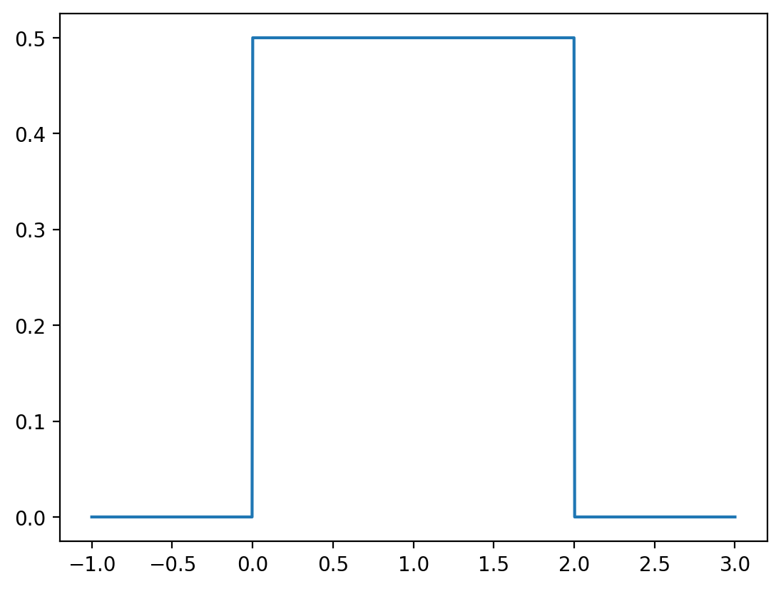
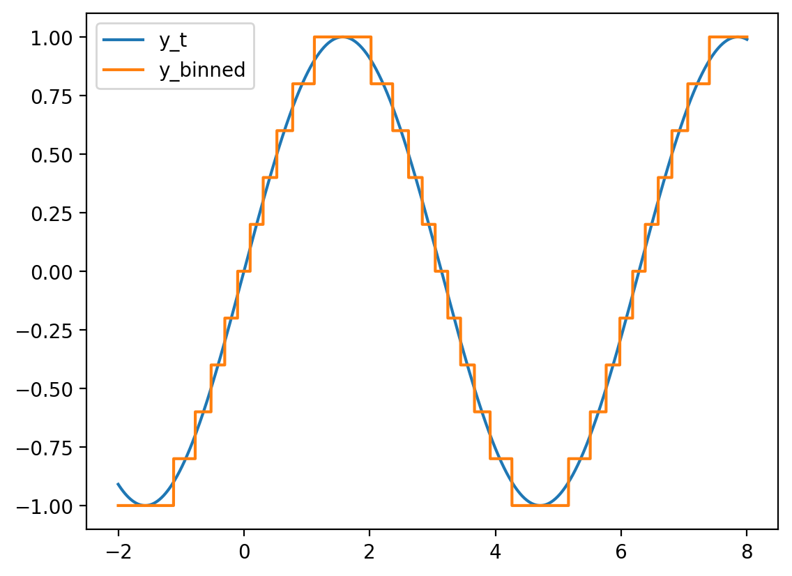
Modeling quantisation error using uniform distribution
Quantization error is the error that arises when representing continuous signals with discrete signals.
NOTE: I am using a simplified convention here. Study DSP for a rigorous treatment (with N and T used in the equations).
Let original signal represented in computer be \(y(t)\). We will quantize the signal to \(x(t)\). The quantization error is given by:
\[ e(t) = y(t) - x(t). \]
We will quantize the signal to \(x(t)\) such that \(x(t)\) can take on \(N\) discrete values. Let \(\Delta\) be the quantization step size. The quantization error is given by:
If the quantization error is uniformly distributed between \(-\Delta/2\) and \(\Delta/2\), then we can model the quantization error as a uniform random variable.
\[ e(t) \sim \text{Uniform}(-\Delta/2, \Delta/2). \]
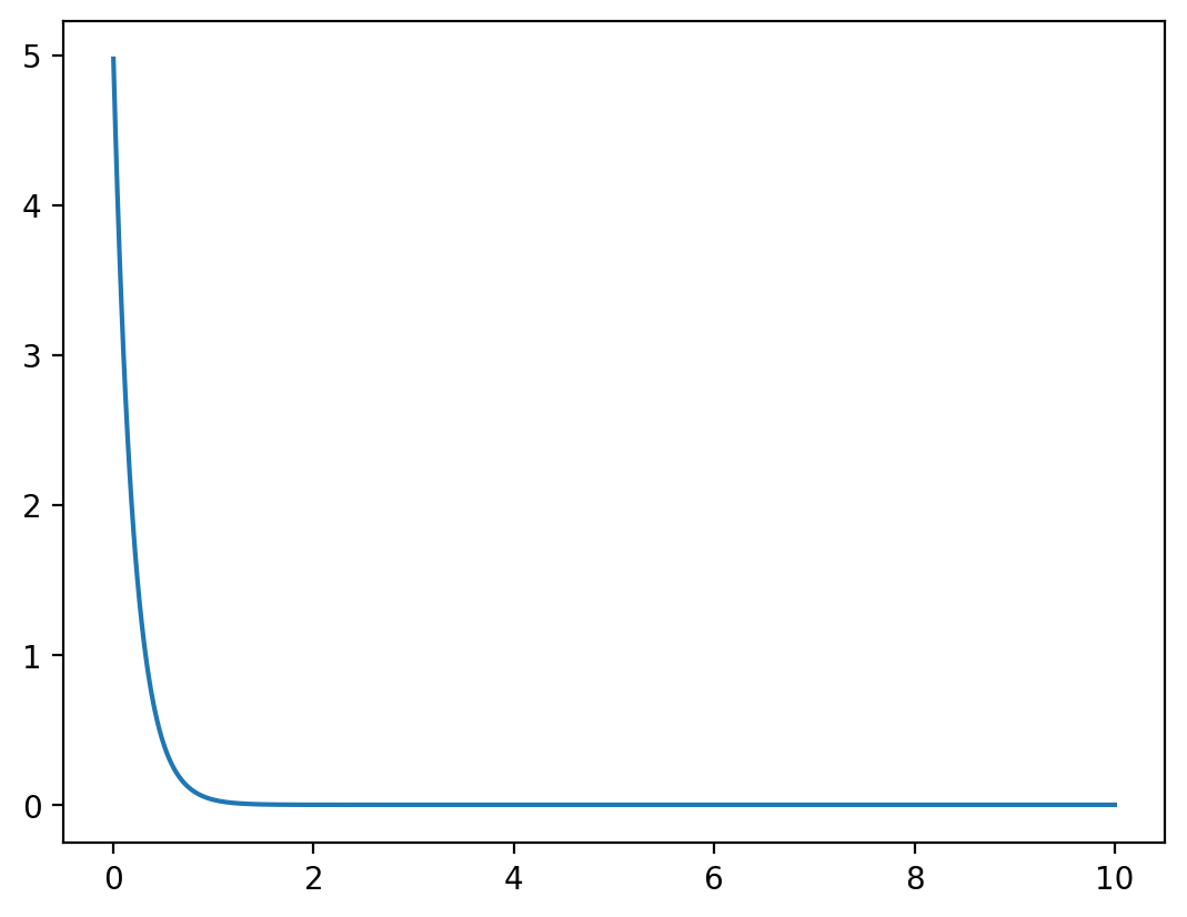
8. Exponential Distribution
The Exponential distribution is the continuous analog of the geometric distribution, modeling the time between events in a Poisson process.
Mathematical Definition
Let \(X \sim \text{Exponential}(\lambda)\) where \(\lambda > 0\) is the rate parameter. The PDF is:
\[f_X(x) = \begin{cases} \lambda e^{-\lambda x} & \text{if } x \geq 0 \\ 0 & \text{otherwise} \end{cases}\]
Properties
- Mean: \(E[X] = \frac{1}{\lambda}\)
- Variance: \(\text{Var}(X) = \frac{1}{\lambda^2}\)
- Support: \([0, \infty)\)
- Memoryless property: \(P(X > s+t | X > s) = P(X > t)\)
- Maximum entropy among distributions with fixed mean on \([0, \infty)\)
Applications
- Reliability engineering (time to failure)
- Queueing theory (service times)
- Radioactive decay
- Phone call durations
- Time between arrivals
Key Insight: Memoryless Property
The exponential distribution is the only continuous distribution with the memoryless property, making it ideal for modeling “fresh start” scenarios.
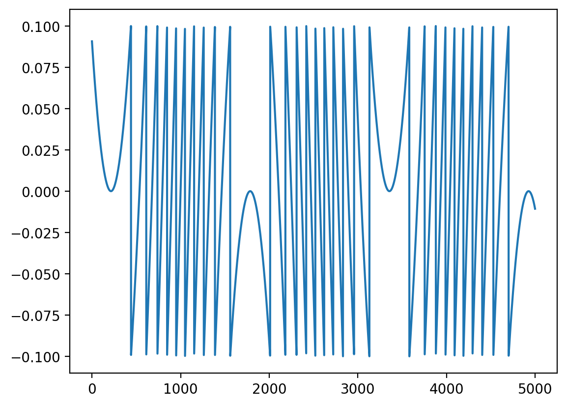
x_t = torch.linspace(-2, 8, 5000)
y_t = torch.sin(x_t)
plt.plot(x_t, y_t, label="y_t")

max_y_t = y_t.max()
min_y_t = y_t.min()

# Divide the range of y_t into N (=10) equal parts
N = 10
y_bins = torch.linspace(min_y_t, max_y_t, N+1)

# Draw the N levels as horizontal lines
for y_level in y_bins:
    plt.axhline(y_level, color='gray', linestyle='--')
    plt.text(3, y_level+.01, f"{y_level:.2f}")

delta = (max_y_t - min_y_t)/N
print(delta)
tensor(0.2000)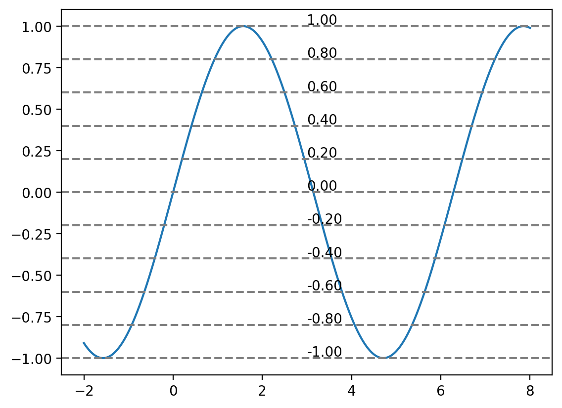
# For x = 3, find the bin in which y_t falls
y_t_x_3 = torch.sin(torch.tensor(3))
print(y_t_x_3)


plt.plot(x_t, y_t, label="y_t")
plt.axvline(3, color='red', linestyle='--')
plt.axhline(y_t_x_3, color='red', linestyle='--')

# Draw the N levels as horizontal lines
for y_level in y_bins:
    plt.axhline(y_level, color='gray', linestyle='--', alpha=0.2)
    plt.text(3, y_level+.01, f"{y_level:.2f}")

# Find the bin in which y_t falls
bin_idx = torch.searchsorted(y_bins, y_t_x_3)
plt.axhline(y_bins[bin_idx], color='green', linestyle='--', label="Closest level")
plt.legend()
tensor(0.1411)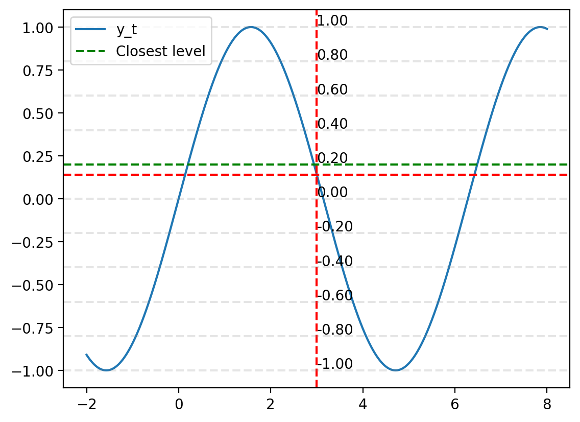
Summary and Practical Guidance
In this comprehensive notebook, we’ve explored the rich world of continuous probability distributions. Each distribution has its unique characteristics and applications:
Distribution Selection Guide
| Data Characteristics | Recommended Distribution | Key Indicators |
|---|---|---|
| Symmetric, bell-shaped | Normal | Central Limit Theorem applies |
| Positive, right-skewed | Log-Normal, Gamma | Multiplicative processes |
| Bounded between 0 and 1 | Beta | Proportions, probabilities |
| Constant over interval | Uniform | Complete uncertainty |
| Waiting times, reliability | Exponential | Memoryless events |
| Heavy tails, robust | Laplace | Outlier resistance needed |
| Positive measurements | Half-Normal | Magnitude of errors |
Key Mathematical Insights
- PDF ≠ Probability: Density functions can exceed 1
- Integration for Probabilities: \(P(a \leq X \leq b) = \int_a^b f(x)dx\)
- Parameter Interpretation: Location, scale, and shape parameters
- Support Matters: Domain restrictions affect model choice
- Maximum Likelihood: Optimal parameter estimation method
Practical Implementation Tips
- Always validate assumptions with data visualization
- Use log-space for numerical stability with small probabilities
- Consider parameter constraints when fitting distributions
- Leverage PyTorch’s automatic differentiation for parameter optimization
- Compare multiple distributions using information criteria (AIC, BIC)
Advanced Topics for Further Study
- Mixture distributions for complex, multi-modal data
- Truncated distributions for bounded domains
- Transformation methods for derived distributions
- Copulas for modeling dependence structures
- Non-parametric methods when distribution assumptions fail
Machine Learning Connections
Continuous distributions are fundamental to: - Variational Autoencoders (VAEs) for latent variable modeling - Generative Adversarial Networks (GANs) for data generation - Bayesian Neural Networks for uncertainty quantification - Gaussian Processes for non-parametric regression - Normalizing Flows for flexible density modeling
Real-World Impact
Understanding continuous distributions enables: - Risk assessment in finance and insurance - Quality control in manufacturing - Signal processing and communications - Epidemiological modeling and public health - Climate science and environmental monitoring
The journey through continuous distributions reveals the mathematical beauty underlying much of our uncertain world. These tools provide the foundation for sophisticated statistical modeling and machine learning applications that impact every aspect of modern data science!
_ = plt.hist(y_t - y_binned, density=True)
plt.xlabel("Error in binning")
plt.ylabel("Density")

theoretical_uniform = torch.distributions.Uniform(-delta/2, delta/2)
x = torch.linspace(-0.1, 0.1, 1000)
x_mask = (x >= -delta/2) & (x <= delta/2)
y = torch.zeros_like(x)
y[x_mask] = theoretical_uniform.log_prob(x[x_mask]).exp()
plt.plot(x, y, label="Theoretical PDF")
plt.legend()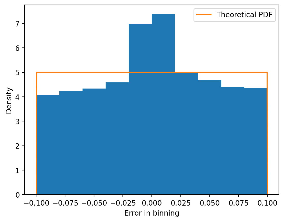
Amount of bits saved
Originally, each sample of the signal was represented using \(B=32\) bits. After quantization, each sample is represented using \(B_q = \log_2(10)\) bits. The amount of bits saved is given by:
\[ (B - B_q) \times \text{number of samples}. \]
from pydub import AudioSegment
import numpy as np

# Load MP3
audio = AudioSegment.from_mp3("vlog-music.mp3")

# Convert to NumPy array
samples = np.array(audio.get_array_of_samples(), dtype=np.float32)
sample_rate = audio.frame_rate

print(f"Samples shape: {samples.shape}")
print(f"Sample rate: {sample_rate}")
Samples shape: (5430528,)
Sample rate: 44100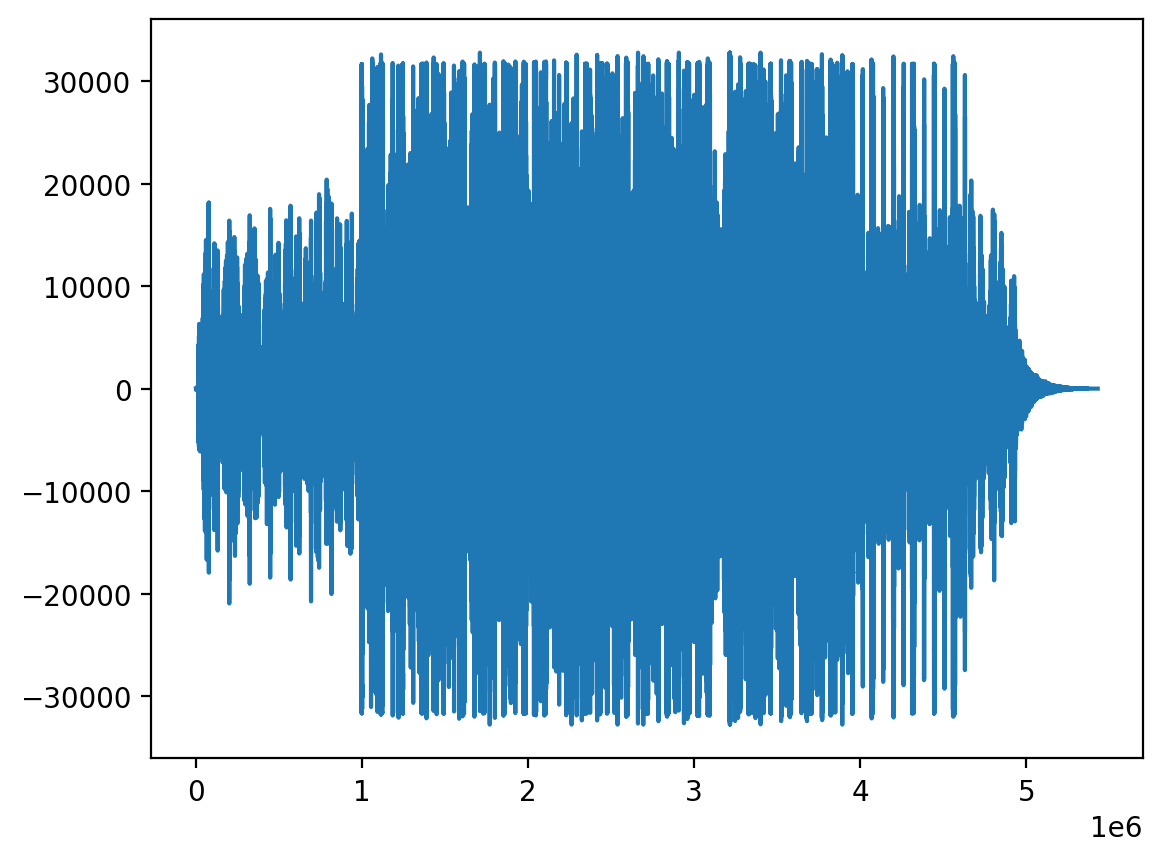
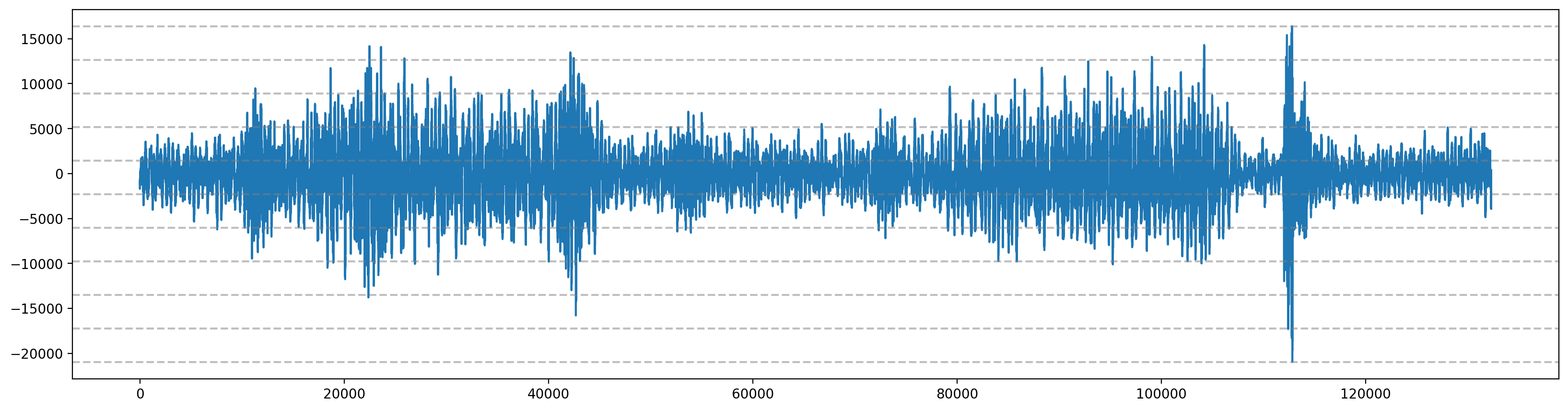
# Plot 2nd second to 5th second
filtered_audio  = samples[sample_rate*2:sample_rate*5]
fig, ax = plt.subplots(figsize=(20, 5))

ax.plot(filtered_audio)

# Quantize to 10 levels
min_audio = filtered_audio.min()
max_audio = filtered_audio.max()

N = 10

audio_bins = torch.linspace(min_audio, max_audio, N+1)
# Plotting audio bins
for audio_bin in audio_bins:
    plt.axhline(audio_bin, color='gray', linestyle='--', alpha=0.5)
# Quantize the audio

audio_bins = np.linspace(min_audio, max_audio, N+1)

# Find closest bin for each audio sample
bins = np.abs(filtered_audio - audio_bins.reshape(-1, 1)).argmin(0)

audio_binned = audio_bins[bins]

fig, ax = plt.subplots(figsize=(20, 5))
ax.plot(filtered_audio, label="Original audio", alpha=0.2)
ax.plot(audio_binned, label="Quantized audio")
ax.legend()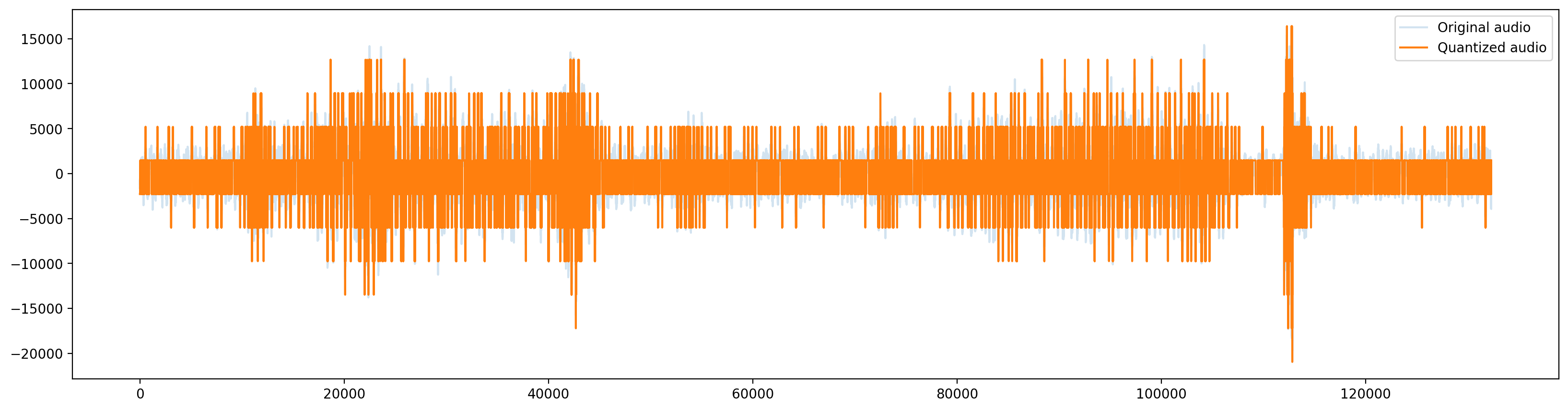
Beta Distribution
Let \(X\) be a random variable that follows a beta distribution with parameters \(\alpha\) and \(\beta\). The probability density function (PDF) of \(X\) is given by:
\[ f_X(x) = \frac{\Gamma(\alpha + \beta)}{\Gamma(\alpha)\Gamma(\beta)} x^{\alpha-1} (1-x)^{\beta-1}, \]
where \(\Gamma(\cdot)\) is the gamma function given as:
\[ \Gamma(z) = \int_0^\infty t^{z-1} e^{-t} dt. \]
We can say that \(X \sim \text{Beta}(\alpha, \beta)\).
Beta distribution is used to model random variables that are constrained to lie within a fixed interval. For example, the probability of success in a Bernoulli trial is a random variable that lies in the interval \([0, 1]\). We can model this probability using a beta distribution.
x_lin = torch.linspace(0.001, 0.999, 1000)
for alpha in range(1, 3):
    for beta in range(1, 3):
        beta_dist = torch.distributions.Beta(alpha, beta)
        y = beta_dist.log_prob(x_lin).exp()
        plt.plot(x_lin, y, label=f"PDF Beta({alpha}, {beta})")

plt.legend()

Exponential Distribution
Let \(X\) be a random variable that follows an exponential distribution with rate parameter \(\lambda\). The probability density function (PDF) of \(X\) is given by:
$$ f_X(x) = \[\begin{cases} \lambda \exp(-\lambda x) & \text{if } x \geq 0, \\ 0 & \text{otherwise}. \end{cases}\]$$
We can say that \(X \sim \text{Exponential}(\lambda)\).
The exponential distribution may be viewed as a continuous counterpart of the geometric distribution, which describes the number of Bernoulli trials necessary for a discrete process to change state. In contrast, the exponential distribution describes the time for a continuous process to change state.